SCRF

Input

Keywords and options specifying details for a PCM calculation (i.e., the default SCRF=PCM or SCRF=CPCM) may be specified in an additional blank-line terminated input section provided that the Read option is also specified. Keywords within this section follow general Gaussian input rules. The available keywords are listed in a separate subsection following the examples.

For the Onsager model (SCRF=Dipole), the solute radius in Angstroms and the dielectric constant of the solvent are read as two free-format real numbers on one line from the input stream. A suitable solute radius is computed by a gas-phase molecular volume calculation (in a separate job step); see the discussion of the Volume keyword.

For the IPCM and SCIPCM models, the input consists of a line specifying the dielectric constant of the solvent and an optional isodensity value (the default for the latter is 0.0004).

Options

Specifying the Solvent

Solvent=item

Selects the solvent in which the calculation is to be performed. Note that the solvent may also be specified in the input stream in various ways for the different SCRF methods. If unspecified, the solvent defaults to water. Item is a solvent name chosen from the list at the end of this section.

Selecting the SCRF Method

PCM

Performs a reaction field calculation using the integral equation formalism model (IEFPCM). This is the default. Some details of the formalism and the implementation have changed with respect to Gaussian 03, as described in [Scalmani10]. IEFPCM is a synonym for PCM.

When PCM is used for an anisotropic or ionic solvent, then items in the PCM input section must be used to select the anisotropic and ionic dielectric models for these types of solvents, using the Read option. The continuous surface charge formalism is also not available with such solvents, and no derivatives can be computed.

CPCM

Performs a PCM calculation using the CPCM polarizable conductor calculation model [Barone98, Cossi03].

Dipole

Performs an Onsager model reaction field calculation.

IPCM

Performs an IPCM model reaction field calculation. Isodensity is a synonym for IPCM.

SCIPCM

Performs an SCIPCM model reaction field calculation, i.e. the SCRF calculation uses a cavity determined self-consistently from an isodensity surface.

SMD Model

SMD

Do an IEFPCM calculation with radii and non-electrostatic terms for Truhlar and coworkers’ SMD solvation model [Marenich09]. This is the recommended choice for computing ΔG of solvation, which accomplished by performing gas phase and SCRF=SMD calculations for the system of interest and taking the difference the resulting energies. You can define a new solvent for use with SMD by providing additional input via the SCRF=Read option (see “Additional Input” for details).

PCM Non-Equilibrium Solvation

NonEquilibrium=action

Save or retrieve data for non-equilibrium solvation. Action is one of the following:

• Save or Write: Save the slow/inertial charges in the checkpoint file (from which they will be retrieved in a subsequent non-equilibrium solvation calculation).
• Read or Load: Read the slow/inertial charges for use in the current non-equilibrium solvation calculation.
• CCSave or CCWrite: Save the slow/inertial correlation charges for use in a subsequent non-equilibrium solvation coupled cluster calculation.
• CCRead or CCLoad: Retrieve the slow/inertial correlation charges for use in the current non-equilibrium solvation coupled cluster calculation.

 

External Iteration PCM

ExternalIteration

Does a self-consistent PCM calculation performing an external iteration through Link 124. This approach computes the energy in solution by making the solute’s electrostatic potential self-consistent with the solvent reaction field [Improta06, Improta07]. ExternalIteration is available only for energy calculations. SelfConsistent and SC are synonyms for this option.

1stVac

Do the first iteration in an external iteration PCM calculation in solution. 1stVac is equivalent to DoVacuum, which is now deprecated.

1stPCM

Do not do the first iteration in an external iteration PCM calculation in solution. 1stPCM is equivalent to SkipVacuum and NoVacuum, which are now deprecated.

Restart

Restarts a PCM external iteration calculation from the checkpoint file.

IEFPCM and CPCM Other Options

SolventAccessibleSurface

For PCM, use a cavity representing the solvent-accessible surface. Only suitable for single-point calculations, but useful for cases with unusual cavities, snapshots from MD with explicit solvent, etc. SCRF=SAS is a synonym for this option.

AsymmetricIEFPCM

Perform asymmetric isotropic IEFPCM rather than the default of symmetric isotropic IEFPCM. AsymmetricIEFPCM was the default in Gaussian 09.
SCRF=AIEFPCM is a synonym for this option. Not valid with CPCM.

PTED

Use the perturbation theory and density approach (PTED) to PCM-CCSD coupling [Cammi09, Caricato12b] for an EOM-CCSD calculation in solution. Other schemes discussed in [Caricato12b] are available via IOp(9/116).

CorrectedLinearResponse

Do a state-specific correction to the energy of a CIS/RPA/TD-DFT SCRF excited state, according to [Caricato06]. CorrectedLR is a synonym for this option.

Read

Indicates that a separate section of keywords and options providing calculation parameters should be read from the input stream. This must be specified for anisotropic and ionic solvents.

Checkpoint

Retrieves the SCRF information from the checkpoint file.

Modify

Retrieves the SCRF information from the checkpoint file, and also reads modifications from the input stream.

ONIOMPCM=k

Performs an ONIOM calculation in solution [Vreven01, Mo04] according to the scheme selected by the code letter k, for which these are the valid values:

A	The reaction field is computed self-consistently using the integrated ONIOM density (available only for energies, and not available for semi-empirical methods).
B	The reaction field is computed for the real-system at the low-level and the corresponding polarization charges are used as external charges in the sub-calculations on the model-systems (available only for energies).
C	The reaction field is computed only for the real-system at the low-level while the sub-calculations on the model-systems are performed assuming zero reaction field (i.e., gas phase). This selection is available for energies, optimizations and frequencies.
X	The reaction field is computed separately in each sub-calculation always using the cavity of the real-system. This is the default if ONIOM and SCRF are specified (available for energies, optimizations and frequencies).

G09Defaults

Sets defaults for PCM solvation back to those used in Gaussian 09.

G03Defaults

Modify the PCM defaults in order to reproduce the results of a Gaussian 03 PCM calculation as closely as possible. Note that perfect agreement is not always possible due to improvements in the program.

Onsager (SCRF=Dipole) Model Options

A0=val

Sets the value for the solute radius a₀ in the route section (rather than reading it from the input stream of an SCRF=Dipole calculation). If this option is included, then Solvent or Dielectric must also be included.

Dielectric=val

Sets the value for the dielectric constant of the solvent. This option overrides Solvent if both are specified.

IPCM Model Options

GradVne

Use Vne basins for the numerical integration.

GradRho

Use density basins for the numerical integration. The job may fail if non-nuclear attractors are present.

SCIPCM Model Options

UseDensity

Force the use of the density matrix in evaluating the density.

UseMOs

Force the use of MOs in evaluating the density.

GasCavity

Use the gas phase isodensity surface to define the cavity rather than solving for the surface self-consistently. This is mainly a debugging option.

Save/Retrieve PCM Charges

SaveQ

Write the PCM charges on the checkpoint file. SaveQ can be specified together with LoadQ. WriteQ is a synonym for this option.

LoadQ

Read the PCM charges on the checkpoint file. Note that the molecular geometry and the cavity must match exactly to use the saved charges. SaveQ can be specified together with LoadQ. ReadQ is a synonym for this option.

Produce Input for COSMO/RS

COSMORS

Produces the data file used by COSMO/RS and other programs.

Availability

The following table details the availability of the various SCRF=PCM calculation types by theoretical method:

Method	Energy (Ext. Iter.)	Energy	Opt	Freq	3rd Order Props a	NMR
MM	no	yes	yes	yes	no	no
AM1, PM3, PM3MM, PM6, PDDG	no	yes	yes	yes	no	no
HF, DFT	yes	yes	yes	yes	yes	yes
MP2	yes	yesb	yesb	yesb	yesb,c	yesb
MP3, MP4(SDQ), CCSD, QCISD	yes	yesb	no	no	no	no
CASSCF	yes	yes	yes	yese	no	no
CIS	yes	yesd	yesd	yesd	no	no
TD	yes	yesd	yesd	yesd	no	no
ZIndo	no	yes	no	no	no	no

^aFor example,Freq=Raman, ROA or VCD; ^bComputed via SCF MO polarization; ^cRaman intensities are computed numerically (i.e., as with Freq=NRaman); ^dUsing the linear response approach; ^eNumerical frequencies only.

CASSCF frequencies with PCM solvation must be done numerically using Freq=Numer.

Restarting SCRF Calculations. SCRF=ExternalIteration and SCRF=IPCM jobs can be restarted from the read-write file by using the Restart option. SCRF=SCIPCM calculations that fail during the SCF iterations should be restarted via the SCF=Restart keyword.

Non-Default Methods. The IPCM model is available for HF, DFT, MP2, MP3, MP4(SDQ), QCISD, CCD, CCSD, CID, and CISD energies only. The SCIPCM model is available for HF and DFT energies and optimizations and numerical frequencies. The Onsager (SCRF=Dipole) model is available for HF, DFT, MP2, MP3, MP4(SDQ), QCISD, CCD, CCSD, CID, and CISD energies, and for HF and DFT optimizations and frequency calculations. However, the Opt Freq keyword combination may not be used in SCRF=Dipole calculations.

Related Keywords

SCF, Volume

Examples

PCM Energy. In general, energy output from the default SCRF method appears in the normal way within the output file. For example, here are the sections of the output file containing the predicted energy from a Hartree-Fock and from an MP2 PCM calculation:

 Hartree-Fock SCRF calculation:
 SCF Done:  E(RHF) =  -99.4687828290     A.U. after    8 cycles
             Convg  =    0.2586D-08             -V/T =  2.0015
 
 MP2 SCRF calculation:			
 E2 =    -0.1192799427D+00  EUMP2 =    -0.99584491345297D+02

The predicted energy in solution includes all computed corrections (unlike in Gaussian 03 output).

Additional output lines may appear when various PCM options are included. For example, the following output is produced by an HF SCRF=SMD calculation:

 SCF Done:  E(RHF) =  -99.4687828290     A.U. after    8 cycles
             Convg  =    0.2586D-08             -V/T =  2.0015
 SMD-CDS (non-electrostatic) energy             (kcal/mol) =       0.54
 (included in total energy above)

For external iteration SCRF calculations, the final energy is computed by Link 124, which controls the external iteration, and is reported in a separate output section, which will appear very near the end of the output file, as in the following example:

 --------------------------------------------------------------------
 Self-consistent PCM results
 ===========================
 <psi(f)|   H    |psi(f)>                     (a.u.) =     -99.577537  (A)
 <psi(f)|H+V(f)/2|psi(f)>                     (a.u.) =     -99.584002  (B)
 (Polarized solute)-Solvent               (kcal/mol) =      -4.06  (C)
 --------------------------------------------------------------------
 Partition over spheres:
 Sphere  on Atom  Surface  Charge   GEl     GCav    GDR
    1      H1      15.27  -0.157   -2.36    0.00    0.00
    2      F2      32.58   0.157   -1.70    0.00    0.00
 --------------------------------------------------------------------
 Predicted energy value for external iteration and state-specific SCRF calculations
 After PCM corrections, the energy is  -99.5840023899     a.u. 
 --------------------------------------------------------------------

Line (A) reports the energy computed using the polarized solute wavefunction and the gas phase Hamiltonian, line (B) reports energy computed using the polarized solute wavefunction and the Hamiltonian in solution, line (C) reports the interaction energy between the polarized solute and the solvent, which corresponds to the integral <Ψ(f)|V(f)/2|Ψ(f)> (in kcal/mol), and the final line reports the predicted energy incorporating all PCM corrections.

Fluorescence example: Emission (Fluorescence) from First Excited State (n→π*) of Acetaldehyde

Here we study the cycle:

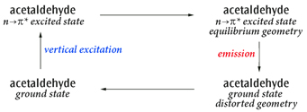
Acetaldehyde Excitation and Emission Cycle

The primary process of interest is the emission, but this example shows how to study the complete cycle including the solvent effects.

Step 1: Ground state geometry optimization and frequencies (equilibrium solvation). This is a standard Opt Freq calculation on the ground state including PCM equilibrium solvation.

%chk=01-ac.chk
# Opt Freq B3LYP/6-31+G(d,p) SCRF=(Solvent=Ethanol) Geom=Connectivity

Acetaldehyde ground state

0 1
C                  1.18859424   -0.14489207    0.00000000
C                 -0.24504511    0.40764331    0.00000000
O                 -1.24669971   -0.28388776    0.00000000
H                  1.17789510   -1.22999932    0.00000000
H                  1.72039616    0.20716276   -0.88008651
H                  1.72039616    0.20716276    0.88008651
H                 -0.30638454    1.51026846    0.00000000

1 2 1.0 4 1.0 5 1.0 6 1.0
2 3 2.0 7 1.0
3
4
5
6
7

Here is the energy of the ground state optimized geometry in solution:

SCF Done:  E(RB3LYP) =  -153.851763001     A.U. after    1 cycles

Step 2: Vertical excitation with linear response solvation. This is a TD-DFT calculation of the vertical excitation with the default solvation, at the ground state equilibrium geometry: i.e., linear response, non-equilibrium. We perform a single-point TD-DFT calculation, which defaults to non-equilibrium solvation. The results of this job will be used to identify which state or states are of interest and their ordering.

%oldchk=01-ac
%chk=02-ac
# B3LYP/6-31+G(d,p) TD=NStates=6 SCRF=(Solvent=Ethanol) Geom=Check Guess=Read

Acetaldehyde absorption: linear response vertical excited states

0 1

The results of the calculation give a reasonable description of the solvation of the excited state, but not quite as good as that from a state-specific solvation calculation. In this case, we see that the n→π* state is the first excited state. Next, we will use the state-specific method to produce a better description of the vertical excitation step.

The vertical excitation (absorption) to first excited state from the non-equilibrium solvation linear response calculation:

Excited State 1: Singlet-A"  4.3767 eV  283.28 nm  f=0.0000  <S**2>=0.000

Thus, the ground state to first excited state absorption is at 283.28 nm (4.38 eV), computed via the linear-response approach.

Step 3: State-specific solvation of the vertical excitation. There are two approaches available for this kind of calculation: Corrected linear-response and External Iteration.

The Corrected linear-response approach is simply a TD-DFT calculation of the vertical excitation at the ground state equilibrium geometry with the non-equilibrium solvation (the default), using the CorrectedLR option:

%oldchk=01-ac
%chk=03-ac
# B3LYP/6-31+G(d,p) TD=(NStates=6,Root=1) Geom=Check Guess=Read
SCRF=(Solvent=Ethanol,CorrectedLR)

Acetaldehyde: Compute energy of the first excited state with
the Corrected linear-response state-specific method and
non-equilibrium solvation

0 1

The predicted vertical excitation (absorption) to first excited state from the non-equilibrium solvation Corrected linear-response calculation appears in the output as follows:

PCM Corrected Linear-Response - Non-equilibrium solvation:
Corrected transition energy               =    4.3603          eV
Total energy after correction             = -153.691525835     a.u.

Thus, the ground state to first excited state absorption is at 284.35 nm (4.36 eV) computed via the Corrected linear-response approach.

For the External Iteration approach, two job steps are required: first, the ground state calculation is done, specifying the NonEquilibrium=Save option, in order to store the information about non-equilibrium solvation based on the ground state. Second, the actual state-specific calculation is done, reading in the necessary information for non-equilibrium solvation using NonEquilibrium=Read option, and specifying the checkpoint file from Step 1:

%oldchk=01-ac
%chk=03-ac-EI
# B3LYP/6-31+G(d,p) SCRF=(Solvent=Ethanol,NonEquilibrium=Save)
  Geom=Check Guess=Read

Acetaldehyde: prepare for state-specific non-eq solvation
by saving the solvent reaction field from the ground state

0 1

--link1--
%chk=03-ac-EI
# B3LYP/6-31+G(d,p) TD(NStates=6,Root=1) Geom=Check Guess=Read
  SCRF=(Solvent=Ethanol,ExternalIteration,NonEquilibrium=Read)

Acetaldehyde: read non-eq solvation from ground state and
compute energy of the first excited with the External Iteration
state-specific method

0 1

Here is the energy of first excited state—at the ground state optimized geometry—from the non-equilibrium solvation state-specific calculation:

After PCM corrections, the energy is  -153.687686675     a.u.

Subtracting this energy from the ground state energy (from step 1) gives the ground state to first excited state absorption including the state-specific solvation correction: at 277.70 nm (4.47 eV).

Step 4: Relaxation of the excited state geometry. Next, we perform a TD-DFT geometry optimization, with equilibrium, linear response solvation, in order to find the minimum energy point on the excited state potential energy surface. Since this is a TD-DFT optimization, the program defaults to equilibrium solvation. As is typical of such cases, the molecule has a plane of symmetry in the ground state but the symmetry is broken in the excited state, so we compute the excited state force constants at the initial geometry (CalcFC) and turn off symmetry (NoSymm). We retrieve the geometry and other data from the checkpoint file from Step 2 to begin the optimisation:

%oldchk=02-ac
%chk=04-ac
# B3LYP/6-31+G(d,p) TD=(NStates=6,Root=1) SCRF=(Solvent=Ethanol)
  Geom=Check Guess=Read Opt=CalcFC Freq NoSymm

Acetaldehyde: excited state opt + freq
Since first excited state is A", the
minimum will break Cs symmetry.

0 1

Here are the results for the first excited state after the geometry optimization of first excited state in solution (equilibrium geometry):

Excited State   1:      Singlet-?Sym    3.2075 eV  386.54 nm  f=0.0014...
      12 -> 13         0.70615
This state for optimization and/or second-order correction.
Total Energy, E(TD-HF/TD-DFT) =  -153.705917055

Note that we included also the calculation of the vibrational frequencies of the excited state (Opt Freq). This way we verified that the geometry located in the excited state optimization job step is a minimum. The results could also be used as part of a Franck-Condon calculation if desired.

Step 5: Emission state-specific solvation Corrected linear-response approach. As for Step 3 above, there are two approaches available for this kind of calculation, Corrected linear-response and External Iteration. We begin with the Corrected linear-response approach. We compute the state-specific equilibrium solvation of the excited state at its equilibrium geometry, writing out the solvation data for the next step via the NonEquilibrium=Save option. Here is the input file:

%oldchk=04-ac
%chk=05-ac
# B3LYP/6-31+G(d,p) TD=(Read,NStates=6,Root=1) Geom=Check Guess=Read
  SCRF=(Solvent=Ethanol,CorrectedLR,NonEquilibrium=Save) NoSymm

Acetaldehyde emission Corrected linear-response
state-specific solvation at first excited state
optimized geometry

0 1

Here is the energy of first excited state—at its optimized geometry—from the equilibrium solvation Corrected linear-response state-specific calculation:

PCM Corrected Linear-Response - Equilibrium solvation:
Corrected transition energy               =    3.1411          eV
Total energy after correction             = -153.708357658     a.u.

Here is the input file for the External Iteration approach:

%oldchk=04-ac
%chk=05-ac-EI
# B3LYP/6-31+G(d,p) TD=(Read,NStates=6,Root=1) Geom=Check Guess=Read
  SCRF=(Solvent=Ethanol,ExternalIteration,NonEquilibrium=Save) NoSymm

Acetaldehyde emission External Iteration
state-specific solvation at first excited state
optimized geometry

0 1

Here is the energy of first excited state—at its optimized geometry—from the equilibrium solvation External Iteration state-specific calculation:

After PCM corrections, the energy is  -153.707149257     a.u.

Step 6: Emission to final ground state. Finally, we compute the ground state energy with non-equalibrium solvation, at the excited state geometry and with the static solvation from the excited state. Using the Corrected linear-response approach, we compute the energy of ground state via a non-equilibrium solvation calculation in solution, using the first excited state optimized geometry and the solvent reaction field in equilibrium with the first excited state density, both read from the results of the previous Corrected liner-response excited state calculation. Here is the input file:

%oldchk=05-ac
%chk=06-ac
# B3LYP/6-31+G(d,p) SCRF=(Solvent=Ethanol,NonEquilibrium=Read)
  Geom=Check Guess=Read NoSymm

Acetaldehyde: ground state non-equilibrium
at excited state geometry.

0 1

SCF Done:  E(RB3LYP) =  -153.822040461     A.U. after   10 cycles

The difference between the energies from steps 5 and 6 gives the vertical emission energy. In this case, the first excited state to ground state emission, including the Corrected linear-response state-specific solvation correction, is at 400.79 nm (3.09 eV).

Here is the input file for the External Iteration approach, which similarly reads the results of the previous calculation:

%oldchk=05-ac-EI
%chk=06-ac-EI
# B3LYP/6-31+G(d,p) SCRF=(Solvent=Ethanol,NonEquilibrium=Read)
  Geom=Check Guess=Read NoSymm

Acetaldehyde: ground state non-equilibrium
at excited state geometry.

0 1

Here is the predicted energy using the External Iteration approach:

SCF Done:  E(RB3LYP) =  -153.822031895     A.U. after   10 cycles

The difference between the energies from steps 5 and 6 gives the vertical emission energy. In this case, the first excited state to ground state emission, including the External Iteration state-specific solvation correction, is at 396.61 nm (3.13 eV).

Steps 1, 2, and 4 would be sufficient to compute the excitation and emission energies in the gas-phase. They are not sufficient when solvent effects are included because the energies computed in step 4 correspond to the ground state solvent reaction field, while the emission takes place in the reaction field created in response to the excited state charge distribution. This is what is accounted for properly in steps 5 and 6.

If the band shape is to be calculated, then in the gas phase one would simply run a calculation with Freq=(ReadFC,FC,Emission), giving the checkpoint file from step 1 as the main checkpoint file for the job, and providing the name of the checkpoint file from step 5 in the input stream to specify the other state. For the solvated band shape, one must do Freq=(ReadFC,FC,Emission,ReadFCHT) using the checkpoint files for steps 1 and 5, but also providing the state-specific emission energy in the input section for the Franck-Condon calculation.

Additional Input

Additional Input for PCM Calculations

Additional input keywords may be specified for PCM SCRF calculations (including ones using the SMD model). Note that many of the available parameters are designed for expert users; experimenting with modifications to the standard settings is strongly discouraged for production calculations.

These keywords are placed in a separate input section, terminated as usual by a blank line, as in this example which tightens the convergence threshold for the iterative calculation of the PCM polarization charges and sets the electrostatic scaling factor for the cavity sphere radii:

# B3LYP/6-31G(d) 5D SCRF(Solvent=Ethanol,Read)
PCM extra input example.
0 1
molecule specification
QConv=10	Input section for PCM keywords
Alpha=1.1
	Blank line terminates PCM input

The PCM input section ends as usual with a blank line.

The available keywords for controlling PCM calculations are listed below, arranged in groups of related items.

Defining Solvent Parameters

The solvent for the PCM calculation is generally specified using the normal Solvent option to the SCRF keyword. You can use the following keywords to override some default values for known solvents.

Eps=x		Specifies the static (or zero-frequency) dielectric constant of the solvent.
EpsInf=x		Specifies the dynamic (or optical) dielectric constant of the solvent. For SMD calculations, it should be set to the square of the solvent’s refractive index at 293 K.
RSolv=x		Specifies the solvent radius (in Angstroms). Relevant only when using AddSph or Surface=SAS.

Unspecified parameters default to the values for the solvent specified with the Solvent option (or to water if this option is omitted).

Defining Solvents for SMD Calculations
The items needed to define a solvent differ for the SMD method. Here is an example of an SMD calculation that defined ethanol manually via a PCM input section. Note that the final five items are SMD-specific keywords. Note that all 7 items are required and that all values must be specified as real numbers. For full details about these parameters, see [Marenich09]. As of this writing, the vast majority of the solvents in the Minnesota Solvent Descriptor Database have solvent keywords defined (see “Solvents”).

# B3LYP/6-31G(d) 5D SCRF(SMD,Solvent=Generic,Read)
Water in solution with ethanol, defined as generic SMD solvent.
0 1
O
H,1,0.94
H,1,0.94,2,104.5
	Input section for PCM keywords
Eps=24.852	ε
EpsInf=1.852593	n2
HbondAcidity=0.37	α
HbondBasicity=0.48	β
SurfaceTensionAtInterface=31.62	γ
CarbonAromaticity=0.	φ
ElectronegativeHalogenicity=0.	ψ
	Blank line terminates PCM input

Calculation Method Variations

NonEq=item		Compute and save the non-equilibrium reaction field after the completion of an HF, DFT or CASSCF calculation using SCRF(Read), or at the end of any SCRF(ExternalIteration,Read) calculation. NonEq=Write says to save the data in the checkpoint file. Use NonEq=Read to retrieve it from the checkpoint file in a subsequent calculation.
Dis		Computes and includes in the total energy the solute-solvent dispersion interaction energy using the model of Floris and Tomasi [Floris89,Floris91]. The default is NoDis. This option cannot be used in a SCRF=SMD calculation.
Rep		Includes the solute-solvent repulsion interaction energy in the total energy using the model of Floris and Tomasi [Floris89,Floris91]. The default is NoRep. This option cannot be used in a SCRF=SMD calculation.
Cav		Includes the solute cavitation energy in the total energy using the model of Pierotti [Pierotti76]. The default is NoCav. This option cannot be used in a SCRF=SMD calculation.
CavityFieldEffects		Includes the effects of the cavity-field interaction energy (also known as local field effect) in the total energy according to the model of Cammi and co-workers [Cammi00a]. The default is not to include this effect.
CF=Eps=x		Specifies a different value for the static dielectric constant to be used in the cavity-field energy contribution. This is useful to modulate the magnitude of the cavity-field effects.
CF=EpsInf=x		Specifies a different value for the dynamic (optical) dielectric constant to be used in the cavity-field energy contribution. This is useful to modulate the magnitude of the cavity-field effects.
FitPot		Performs analysis of the solute-solvent interaction energy in terms of atomic or atomic groups additive contributions. This analysis involves a fitting of atomic charges to the molecular electrostatic potential in solution.
Iterative		Solves the PCM electrostatic problem to calculate polarization charges through an iterative method.
MxIter=N		Specifies the maximum number of iterations allowed to the iterative solution of the electrostatic problem. 400 is the default.
QConv=type|N		Sets the convergence threshold for the iterative calculations of the PCM polarization charges to 10-N or to one of the following predefined types: VeryTight (10-12), Tight (10-9) and Sleazy (10-6). The default is QConv=Tight.
SC=QConv=x		Specifies the convergence for the PCM polarization charges during the external iteration procedure.
MaxExtIt=x		Specify the maximum number of iterations allowed during the external iteration procedure.

Anisotropic and Ionic Solvents

Anisotropic		Performs a PCM calculation for an anisotropic solvent according to the IEFPCM formalism. The 3-rank symmetric tensor representing the dielectric constant must be specified as the values for these six additional keywords: EPSX, EPSY, EPSZ, EUPHI, EUTHE, and EUPSI (all of them take a parameter: e.g., EPSX=value).
Ionic		Performs a PCM calculation for ionic solution according to the IEFPCM formalism. The ionic strength in mol/dm3 has to be specified as the value to the keyword DISM.

Specifying the Molecular Cavity

By default, the program builds up the cavity using the UFF radii, which places a sphere around each solute atom, with the radii scaled by a factor of 1.1. There are also three United Atom (UA) models available.

The cavity can be extensively modified in the PCM input section: changing sphere parameters and the general cavity topology, adding extra spheres to the cavity built by default, and so on. The whole molecular cavity can be also provided by the user in the input section.

Radii=model: Indicates the topological model and/or the set of atomic radii used. Available models and sets are:

• UFF: Uses radii from the UFF force field. Hydrogens have individual spheres (explicit hydrogens). This is the default.
• UA0:Uses the United Atom Topological Model applied on atomic radii of the UFF force field for heavy atoms. Hydrogens are enclosed in the sphere of the heavy atom to which they are bonded. This was the default in Gaussian 03.
• UAHF: Uses the United Atom Topological Model applied on radii optimized for the HF/6-31G(d) level of theory.
• UAKS: Uses the United Atom Topological Model applied on radii optimized for the PBE1PBE/6-31G(d) level of theory.
• Pauling: Uses the Pauling (actually Merz-Kollman) atomic radii (uses explicit hydrogens).
• Bondi: Uses the Bondi atomic radii (uses explicit hydrogens).

Surface=type: Specify the type of molecular surface representing the solute-solvent boundary. Available options are:

• VDW: Van der Waals surface. Uses atomic radii (scaled) and skips the generation of “added spheres” to smooth the surface. This is the default.
• SES: Solvent Excluding Surface. The surface is generated by the atomic or group spheres and by the spheres created automatically to smooth the surface (“added spheres”). This was the default in Gaussian 03.
• SAS: Solvent Accessible Surface. The radius of the solvent is added to the unscaled radii of atoms and/or atomic groups.

ModifySph: Alters parameters for one or more spheres. The modified spheres can be indicated in the PCM input in lines following this keyword having the following format:

   atom radius [alpha]

where atom is the atom number or element type.

ExtraSph=N: Adds N user-defined spheres to the cavity. Parameters of the spheres can be specified in lines following this keyword using the following format:

   X Y Z radius [alpha]

where X,Y,Z are the Cartesian coordinates in the standard orientation.

NSph=N: The cavity is built just from the N spheres provided by the user, specified on lines of the following format:

   atom_number radius [alpha] —or— X Y Z radius [alpha]

where X,Y,Z are the Cartesian coordinates in the standard orientation. Specifying spheres by atom number mimics standard cavity behavior, while specifying Cartesian produces a fixed cavity which does not move with the structure.

PDens=x		Sets the average density of integration points on the surface, in units of Angstrom-2. 5.0 is the default. Increasing this value results in a finer surface discretization.
Alpha=scale		Specifies the electrostatic scaling factor by which the sphere radius is multiplied. The default value is 1.1.
SphereOnH=N		When using a United Atom Topological model, places an individual sphere on the hydrogen at the Nth position in the atoms list.
SphereOnAcidicHydrogens		When using a United Atom Topological model, puts individual spheres on acidic hydrogens (those bonded to N, O, S, P, Cl and F atoms).
OFac=x		Specifies the overlap index between two interlocking spheres [Pascual-Ahuir94] for SES added spheres. Decreasing this index results in a smaller number of added spheres. The default value is 0.89.
RMin=x		Sets the minimum radius in Angstroms for SES added spheres. Increasing this value results in a smaller number of added spheres. The default value is 0.2.
PrintSpheres		Include solvation cavity data within the checkpoint file for later visualization with GaussView.
GeomView		Create the file points.off describing the cavity. This file contains input for the GeomView program (see www.geomview.org), which can be used to visualize the molecular cavity.