


How do I generate Natural Transition Orbitals?
The TD-DFT method in Gaussian makes it practical to study excited state systems since it produces results that are comparable in accuracy to ground state DFT calculations. Sometimes, characterizing the specific transition associated with an excited state is straightforward. In other instances, however, the state may be described by a substantial list of orbital transitions with coefficients that are similar in magnitude, without any single dominant component.
Natural transition orbitals (NTOs) can be a helpful way of obtaining a qualitative description of electronic excitations. They do so by transforming the ordinary orbital representation into a more compact form in which each excited state is expressed as a single pair of orbitals (if possible): the NTO transition occurs from excited particle (occupied) to the empty hole (unoccupied). See [Martin03] for a detailed description of natural transition orbitals.
Gaussian Jobs for Generating NTOs
You can generate NTOs via these steps:
- Run an excited state calculation, saving the checkpoint file.
- Examine the calculation results to determine the excited state of interest.
- Run a single point calculation to generate the NTOs for the desired excited state.
The third step can be repeated for each excited state in which you are interested.
Here is an example input file for the first step. It is a TD-DFT calculation on a molecular structure that we have previously optimized and verified as a minimum:
%Chk=tddft
# B3LYP/6-311+G(2d,p) TD(NStates=40)
TD-DFT excited state calculation: B3LYP/6-311+G(2d,p)

molecule specification
Now we need to run a second calculation to generate and save the NTOs for visualization in GaussView or another graphics package. In this example, we compute the NTOs for the third excited state:
%OldChk=tddft
%Chk=state3
# B3LYP/6-311+G(2d,p) Geom=AllCheck Guess=(Read,Only) Density=(Check,Transition=3) Pop=(Minimal,NTO,SaveNTO)
NTOs are generated when the Pop=NTO option is specified. The Pop=SaveNTO option tells Gaussian to replace the ground state orbitals normally in the checkpoint file with the computed NTOs. GaussView and other graphics packages will visualize whatever orbitals are present in the checkpoint file, so no special handling is required inside the visualization program.
Note that we use a separate checkpoint file for the NTOs. If you plan to compute the NTOs for multiple states, use a different checkpoint file for each state. For example, the following second job step within the preceding input file will generate and save the NTOs for the sixth excited state:
--Link1--
%OldChk=tddft
%Chk=state6
# B3LYP/6-311+G(2d,p) Geom=AllCheck Guess=(Read,Only) Density=(Check,Transition=6) Pop=(Minimal,NTO,SaveNTO)
The %OldChk command was introduced in G09 Rev C.01. It copies information from the old checkpoint file (tddft.chk) to a new checkpoint file (state3.chk) and uses the latter for the current calculation. If you are using an older version of Gaussian, you should manually copy the checkpoint file to a new name before the second generating the NTOs; you will use the name of the copy as the checkpoint file in the second job.
Example: Pt(dcbpy)Cl2
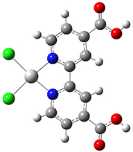
We will consider the 19th excited state of Pt(dcbpy)Cl2 as an example (see [Roy09] for details about this compound). Here is the output from a TD-DFT calculation on this compound:
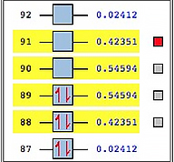
Excited State 19: Singlet-A 4.7936 eV 258.64 nm f=0.0002 …
78 -> 90     0.41835
78 -> 92    -0.18686
78 -> 95     0.17948
79 -> 91     0.42043
79 -> 94    -0.10009
79 -> 99     0.12527
80 -> 90     0.15807
87 -> 92     0.11388
The component transitions of this excited state are numerous, and no one or two transitions is decisively dominant. The following figure shows the relevant molecular orbitals and transitions, labeling each with the corresponding coefficient:
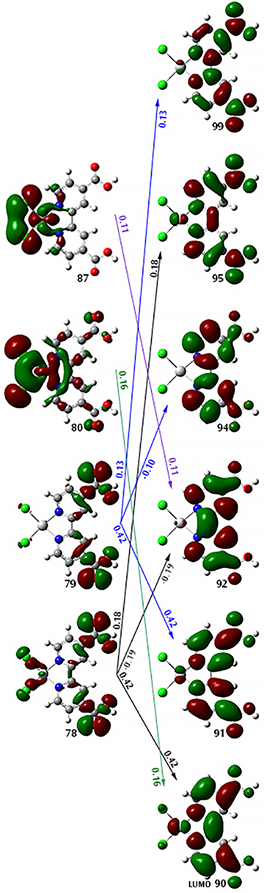
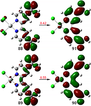
When we compute the NTOs for this state, we obtain two pairs. This greatly simplifies the process of characterizing this transition.
Calculation details: TD(NStates=40) CAM-B3LYP/Gen Pseudo=Read; basis set/ECPs: 6-311G(d) with LANL08 for Pt.
References
[Martin03] Martin, R. L. “Natural transition orbitals.” JCP 2003, 118, 4775-4777. doi:10.1063/1.1558471
[Roy09] Roy, L. E.; Scalmani, G.; Kobayashi, R.; Batista, E. R.“Theoretical studies on the stability of molecular platinum catalysts for hydrogen production.” Dalton Trans. 2009, 6719–6721. doi:10.1039/b911019b
Last updated on: 14 August 2016.