


Antiferromagnetic coupling is an effect that is often important for molecules with high spin multiplicity like this bridged manganese complex:
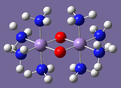
This is a typical transition metal system in which antiferromagnetic coupling is of interest: Mn2O2(NH3)8. In the netural molecule, in which the Mn atoms are nominally Mn(II), there are 5 d electrons on each Mn, and the antiferromagnetic singlet (5 alpha d electrons on one Mn and 5 beta d electrons on the other) may be the ground state. The cations Mn2O2(NH3)8n+ (n=1-4) are also of interest and may also have antiferromagnetic ground states.
In doing computations on this set of molecules, it is easiest to start with the system having half-filled d shells (in this case, the neutral). The rationale behind this approach is that because the charged systems with partially filled d shells give rise to additional issues of symmetry breaking in both the wavefunction and in the geometry. So it is best to do the filled case first, and then use its orbitals as the initial guess for the other cases.
Building the Molecule in GaussView
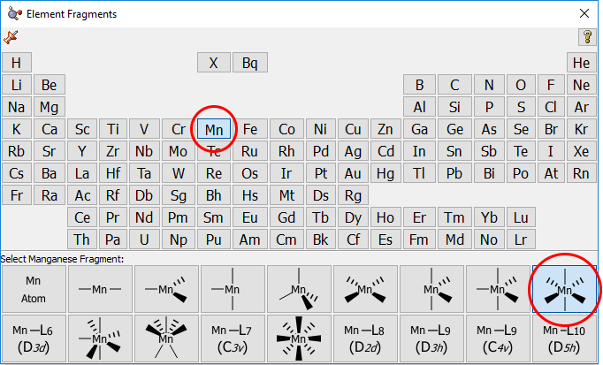
This molecule can have D2h symmetry, so it is best to start the optimization from this high symmetry configuration. First, we sketch the molecule in GaussView, starting with an octahedral Mn atom, selected from the Element panel:
We next replace two hydrogens with oxygens and then add the other Mn atom as a separate fragment. We then move it into its approximate position by holding down the Alt key while dragging it.
Next, we check the Mn-O bond distance (before deleting the hydrogens) using Inquire mode:
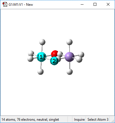
The bond distance is display at the bottom of the window. We note that is it 1.83 Angstroms.
We go on to delete the two unneeded hydrogens on the second Mn atom, and then create the bonds between this atom and each oxygen atom, setting the bond distance to be 1.83 Angstroms. Once this is completed, we use the Clean function to regularize the geometry.
At this point, it is helpful to use GaussView’s Edit Point Group dialog to ensure that the resulting Mn2O2H8 system has D2h symmetry. We open the dialog (via the Tools=>Point Group menu path), and check Enable Point Group Symmetry. We change the tolerance to Do you feel lucky?, and select D2h from the popup menu in the Approximate higher-order point groups section. Then we click the Symmetrize button to impose this point group on the structure:
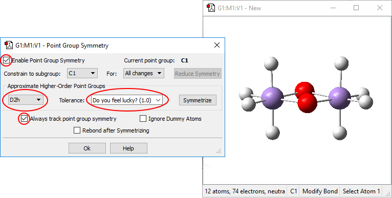
If D2h is not a selection listed in the popup menu when you build this molecule, symmetrize the molecule to the highest listed point group and them examine it in Inquire mode. You may need to adjust some bond or dihedral angles manually in order for D2h symmetry to be recognized. Note that this issue is more likely to occur with GV4 than with GV5.
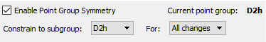
Before leaving the Point Group Symmetry dialog, we set the Constrain to subgroup menu to D2h and click Always track point group symmetry:
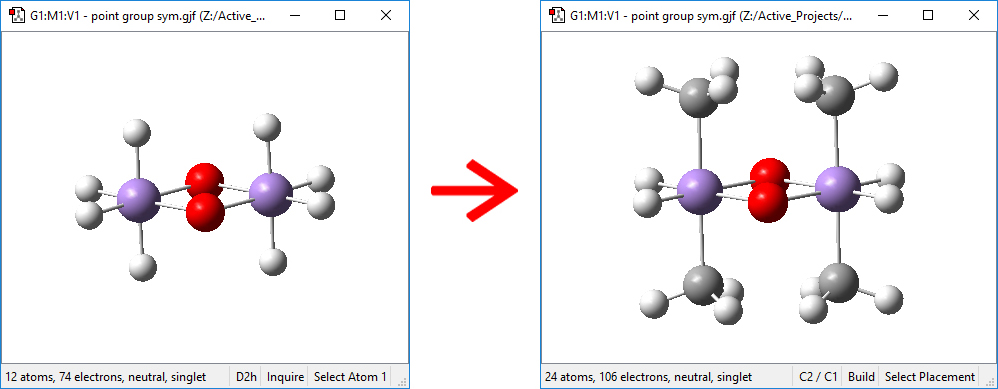
The next step in building the molecule is to replace the hydrogens with CH3 groups. First, we replace the four hydrogens which are above and below the plane of the heavy atoms. We select the appropriate C hybridization and then click on one of the hydrogen atoms:
Note that the symmetry constraints result in all four CH3 groups being added in one operation. You might need to use the Point Group Symmetry dialog to return the molecule to D2h symmetry after this step.
Once this is completed, go on to replace the other four hydrogen atoms with methyl groups. In this case, you will very likely need to adjust dihedral atoms to rotate the new methyl groups in order to achieve D2h symmetry. Typically, you will need to set the dihedral angle for the hydrogen atom pointing out of the plane of the screen/paper to 0 degrees:
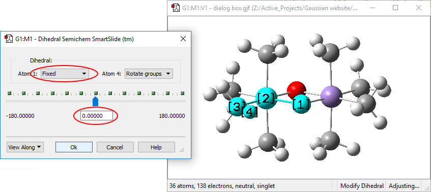
Note that you must be sure to set the action for Atom 1 to Fixed to constrain movement in the molecule to rotation of the methyl group.
The final step is to replace the carbon atoms with nitrogens, and then impose D2h symmetry one final time to produce the final input structure.
Running the Calculations
We ran sequence of calculations to find the optimal geometry and wavefunction for the high spin state (multiplicity 11), followed by use of the resulting wavefunction as the initial guess for the antiferromagnetic singlet.
Job 1: Here we optimize the structure for the high spin state from the input generated with GaussView. We can use the GaussView Gaussian Calculation Setup dialog to perform most of the work:
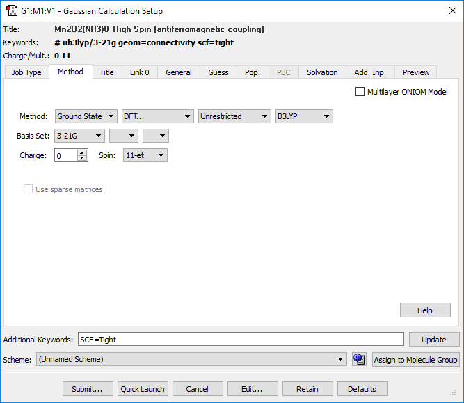
We specify a geometry optimization using the UB3LYP/3-21G model chemistry. We set the Spin to 11-et. Once we have made all of the appropriate selections, we can then submit it to Gaussian.
Note: When we actually ran this job, we also included additional directives in the route section specifying memory and the desired number of processors. Be aware that it requires nontrivial computational resources.
Job 2: Next, we check the stability of the wavefunction at the final geometry. Here is the input file:
%oldchk=afc1 %chk=afc2 #p b3lyp/3-21g guess=read geom=check stable=opt Mn2O2(NH3)8 High Spin (antiferromagnetic coupling) 0,11 |
Note: We make a copy of the checkpoint file from the first job prior to running this job, naming it afc2. We choose to do this before each job in order to be able to return to an earlier step in the sequence if desired.
As we suspected would be the case, a lower energy high spin state was found by the Stable=Opt job. The presence of an unstable wavefunction is indicated by lines like these in the output file:
 ***********************************************************************
Stability analysis using <AA,BB:AA,BB> singles matrix:
***********************************************************************
Eigenvectors of the stability matrix:
Eigenvector 1: ?Spin -B2G Eigenvalue=-0.0129755
75A -> 79A 0.68583
76A -> 80A 0.70288
Eigenvector 2: ?Spin -B1U Eigenvalue=-0.0066257
70A -> 79A -0.10926
75A -> 80A 0.37604
76A -> 79A 0.89115
Eigenvector 3: ?Spin -B3U Eigenvalue= 0.0058150
77A -> 80A -0.34398
78A -> 79A 0.92278
The wavefunction has an internal instability.
|
The job succeeds in finding a lower energy stable wavefunction.
Job 3. The next step is to reoptimize the high spin geometry using the better high spin wavefunction, using the following input file:
%oldchk=afc2 %chk=afc3 #p b3lyp/3-21g opt geom=allcheck guess=read |
The optimization succeeded.
Job 4: Check the stability of the high-spin wavefunction at the final geometry of the second optimization. Here is the input file:
%oldchk=afc3 %chk=afc4 # b3lyp/3-21g guess=read geom=allcheck stable=opt |
The wavefunction was confirmed to be stable.
Job 5: Now we set up a fragment guess job. Previously, we had to go to considerable effort to set up the initial guess for the antiferromagnetic singlet. Now, with Gaussian 16’s fragment guess features and GaussView 6 fragment support, it is very quick and easy.
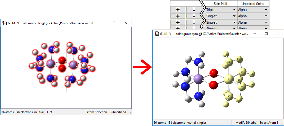
In GaussView 6, using the optimized high-spin geometry, we define 4 fragments using the Atom Groups Editor (Tools=>Atom Groups menu path). We select Gaussian Fragment in the Atom Group Class popup in the upper left of the dialog. Initially, the panel shows one fragment containing all of the atoms in the molecule. we begin by creating three more fragments using the New Group in the Group Actions menu at the upper right. Next, we will place one of the Mn atoms and its attached NH3 groups into fragment 2. We hold down the R key and drag a marquee around the desired atoms to select them, and then click on the + button under Selected Atoms on the far right end of the Gaussian Fragment (2) row in the table:
We select each oxygen atom and place it into its own fragment. We assign charges of -2 to each oxygen atom fragment and +2 to each Mn(NH3)4 fragment. We specify each of the latter fragments to be a sextet. Finally, we define one of the latter fragments asw having Beta spin. The Atom Group Editor will now look like this:
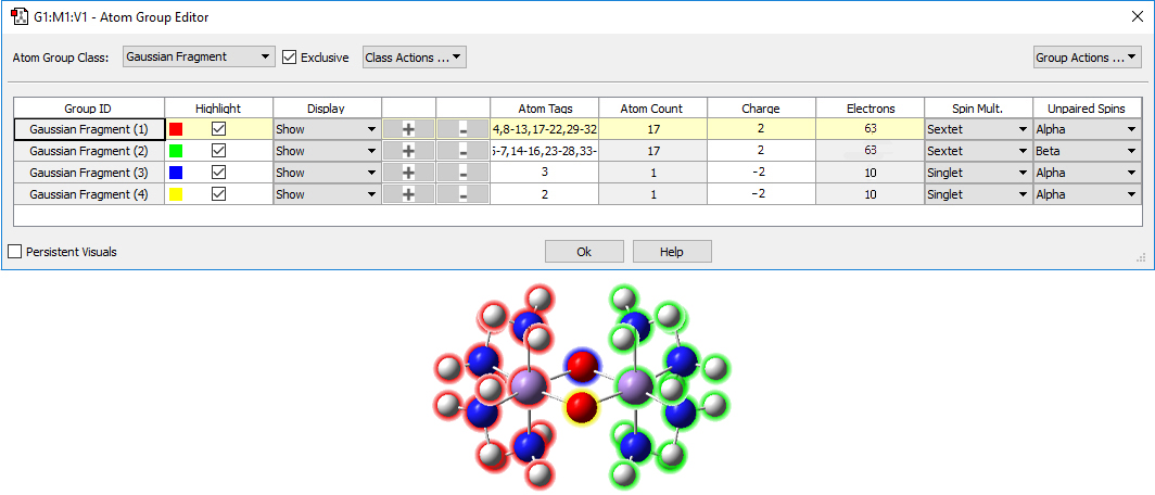
We have also turned on highlighting in the molecule display.
Next, we open the Gaussian Calculation Setup dialog, and set up the fragment guess job. GaussView has already entered our fragment-specific charges and spin multiplicities into the molecule specification. We endure that Use fragment (atom group) for generating guess and Only do guess (no SCF) are checked in the Guess panel. Here is the route of the resulting job:
%oldchk=afc4 %chk=afc5 # ub3lyp/3-21g guess=(fragment=4,only) |
Job 6: We finally perform a stabilty calculation on the resulting wavefunction and confirm that it is stable. Here is the route section:
%oldchk=afc5 %chk=afc6 # ub3lyp/3-21g scf=nosymm guess=read geom=allcheck stable=opt |
The job produces a wavefunction which has a reasonable energy and predicts spin densities of about +4 on one Mn and -4 on the other. The spin densities aren’t expected to be exactly 5 on each metal, because some of the spin density delocalizes onto the ligands, so this is a reasonable result for antiferromagnetic coupling of 10 electrons.
Here is the relevant part of the output file:
Mulliken atomic spin densities:
              1
     1  Mn   3.931283
     2  O   -0.000000
     3  O   -0.000000
     4  Mn  -3.931283
     5  H    0.005293
     ...
|
Results and Summary
As a check, we also did a Stable=Opt calculation starting from the closed-shell singlet (Job 7). Since G09 Rev. D.01, “Stable=Opt” starting from closed-shell singlet is able to get to the antiferromagnetic solution in this case. The closed-shell singlet was unstable, as expected, and a subsequent Stable=Opt found a wavefunction with Sz=0 which was lower in energy than the closed shell but not as low as the antiferromagnetic one, consistent with the antiferromagnetic state being the ground state.
Here is the route section we used for this job:
%oldchk=afc5 %chk=afc7 #p rb3lyp/3-21g geom=allcheck stable=opt |
The following table summarizes the energies of the various states we studied:
| State | Gaussian Job | Wavefunction Stable? |
Energy
|
| Spin=11 | Job 1 (Opt) | no |
-2890.79483366
|
| Spin=11 | Job 2 (Stable=Opt) | yes |
-2890.81173654
|
| Spin=11 | Job 3 (Opt) | yes (confirmed by Job 4) |
-2890.86435160
|
| Antiferromagnetic Singlet | Job 6 (Stable=Opt) | yes |
-2890.87105285
|
| Closed Shell Singlet | Job 7 Stable=Opt | yes (but next job reveals RHF-UHF instability) |
-2890.62426589
|
| Open Shell Singlet | Stable=Opt | yes |
-2890.77534535
|
Last updated on: 6 September 2022.