


Joseph W. Ochterski, Ph.D.
help@gaussian.com
October 29, 1999
Minor updates: 17 June 2018, 20 August 2020
Get PDF file of this paper (you may need to Right-Click this link to download it).
Abstract
One of the most commonly asked questions about Gaussian is “What is the definition of reduced mass that Gaussian uses, and why is is different than what I calculate for diatomics by hand?” The purpose of this document is to describe how Gaussian calculates the reduced mass, frequencies, force constants, and normal coordinates which are printed out at the end of a frequency calculation.
Contents
The Short Answer
So why is the reduced mass different in Gaussian? The short answer is that Gaussian uses a coordinate system where the normalized cartesian displacement is one unit. This differs from the coordinate system used in most texts, where a unit step of one is used for the change in interatomic distance (in a diatomic). The vibrational analysis of polyatomics in Gaussian is not different from that described in “Molecular Vibrations” by Wilson, Decius and Cross. Diatomics are simply treated the same way as polyatomics, rather than using a different coordinate system.
The Long Answer
In this section, I’ll describe exactly how frequencies, force constants, normal modes and reduced mass are calculated in Gaussian, starting with the Hessian, or second derivative matrix. I’ll outline the general polyatomic case, leaving out details for dealing with frozen atoms, hindered rotors, and the like.
I will try to stick close to the notation used in “Molecular Vibrations” by Wilson, Decius and Cross. I will add some subscripts to indicate which coordinate system the matrix is in.
There is an important point worth mentioning before starting. Vibrational analysis, as it’s descibed in most texts and implemented in Gaussian, is valid only when the first derivatives of the energy with respect to displacement of the atoms are zero. In other words, the geometry used for vibrational analysis must be optimized at the same level of theory and with the same basis set that the second derivatives were generated with. Analysis at transition states and higher order saddle points is also valid. Other geometries are not valid. (There are certain exceptions, such as analysis along an IRC, where the non-zero derivative can be projected out.) For example, calculating frequencies using HF/6-31g* on MP2/6-31G* geometries is not well defined.
Another point that is sometimes overlooked is that frequency calculations need to be performed with a method suitable for describing the particular molecule being studied. For example, a single reference method, such as Hartree-Fock (HF) theory is not capable of describing a molecule that needs a multireference method. One case that comes to mind is molecules which are in a ![]() ground state. Using a single reference method will yield different frequencies for the
ground state. Using a single reference method will yield different frequencies for the ![]() and
and ![]() vibrations, while a multireference method shows the cylindrical symmetry you might expect. This is seldom a large problem, since the frequencies of the other modes, like the stretching mode, are are still useful.
vibrations, while a multireference method shows the cylindrical symmetry you might expect. This is seldom a large problem, since the frequencies of the other modes, like the stretching mode, are are still useful.
Mass weight the Hessian and diagonalize
We start with the Hessian matrix ![]() , which holds the second partial derivatives of the potential V with respect to displacement of the atoms in cartesian coordinates (CART):
, which holds the second partial derivatives of the potential V with respect to displacement of the atoms in cartesian coordinates (CART):
![]()
This is a ![]() matrix (N is the number of atoms), where
matrix (N is the number of atoms), where ![]() are used for the displacements in cartesian coordinates,
are used for the displacements in cartesian coordinates, ![]() . The
. The ![]() refers to the fact that the derivatives are taken at the equilibrium positions of the atoms, and that the first derivatives are zero.
refers to the fact that the derivatives are taken at the equilibrium positions of the atoms, and that the first derivatives are zero.
The first thing that Gaussian does with these force constants is to convert them to mass weighted cartesian coordinates (MWC).
![]()
where ![]() ,
, ![]() and so on, are the mass weighted cartesian coordinates.
and so on, are the mass weighted cartesian coordinates.
A copy of ![]() is diagonalized, yielding a set of 3N eigenvectors and 3Neigenvalues. The eigenvectors, which are the normal modes, are discarded; they will be calculated again after the rotation and translation modes are separated out. The roots of the eigenvalues are the fundamental frequencies of the molecule. Gaussian converts them to cm
is diagonalized, yielding a set of 3N eigenvectors and 3Neigenvalues. The eigenvectors, which are the normal modes, are discarded; they will be calculated again after the rotation and translation modes are separated out. The roots of the eigenvalues are the fundamental frequencies of the molecule. Gaussian converts them to cm ![]() , then prints out the 3N (up to 9) lowest. The output for water HF/3-21G* looks like this:
, then prints out the 3N (up to 9) lowest. The output for water HF/3-21G* looks like this:
Full mass-weighted force constant matrix:
 Low frequencies ---   -0.0008    0.0003    0.0013   40.6275   59.3808   66.4408
 Low frequencies --- 1799.1892 3809.4604 3943.3536
In general, the frequencies for for rotation and translation modes should be close to zero. If you have optimized to a transition state, or to a higher order saddle point, then there will be some negative frequencies which may be listed before the “zero frequency” modes. (Freqencies which are printed out as negative are really imaginary; the minus sign is simply a flag to indicate that this is an imaginary frequency.) There is a discussion about how close to zero is close enough, and what to do if you are not close enough in Section 4 of this paper.
You should compare the lowest real frequencies list in this part of the output with the corresponding frequencies later in the output. The later frequencies are calculated after projecting out the translational and rotational modes. If the corresponding frequencies in both places are not the same, then this is an indication that these modes are contaminated by the rotational and translational modes.
Determine the principal axes of inertia
The next step is to translate the center of mass to the origin, and determine the moments and products of inertia, with the goal of finding the matrix that diagonalizes the moment of inertia tensor. Using this matrix we can find the vectors corresponding to the rotations and translations. Once these vectors are known, we know that the rest of the normal modes are vibrations, so we can distinguish low frequency vibrational modes from rotational and translational modes.
The center of mass ( ![]() ) is found in the usual way:
) is found in the usual way:
![]()
where the sums are over the atoms, ![]() . The origin is then shifted to the center of mass
. The origin is then shifted to the center of mass ![]() . Next we have to calculate the moments of inertia (the diagonal elements) and the products of inertia (off diagonal elements) of the moment of inertia tensor (
. Next we have to calculate the moments of inertia (the diagonal elements) and the products of inertia (off diagonal elements) of the moment of inertia tensor ( ![]() ).
).

This symmetric matrix is diagonalized, yielding the principal moments (the eigenvalues ![]() ) and a
) and a ![]() matrix (
matrix ( ![]() ), which is made up of the normalized eigenvectors of
), which is made up of the normalized eigenvectors of ![]() . The eigenvectors of the moment of inertia tensor are used to generate the vectors corresponding to translation and infinitesimal rotation of the molecule in the next step.
. The eigenvectors of the moment of inertia tensor are used to generate the vectors corresponding to translation and infinitesimal rotation of the molecule in the next step.
Generate coordinates in the rotating and translating frame
The main goal in this section is to generate the transformation ![]() from mass weighted cartesian coordinates to a set of 3N coordinates where rotation and translation of the molecule are separated out, leaving 3N-6 or 3N-5 modes for vibrational analysis. The rest of this section describes how the Sayvetz conditions are used to generate the translation and rotation vectors.
from mass weighted cartesian coordinates to a set of 3N coordinates where rotation and translation of the molecule are separated out, leaving 3N-6 or 3N-5 modes for vibrational analysis. The rest of this section describes how the Sayvetz conditions are used to generate the translation and rotation vectors.
The three vectors ( ![]() ,
, ![]() ,
, ![]() ) of length 3N corresponding to translation are trivial to generate in cartesian coordinates. They are just
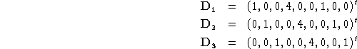
) of length 3N corresponding to translation are trivial to generate in cartesian coordinates. They are just ![]() times the corresponding coordinate axis. For example, for water (using
times the corresponding coordinate axis. For example, for water (using ![]() and
and ![]() ) the translational vectors are:
) the translational vectors are:
Generating vectors corresponding to rotational motion of the atoms in cartesian coordinates is a bit more complicated. The vectors for these are defined this way:
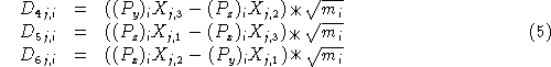
where j=x, y, z; i is over all atoms and P is the dot product of ![]() (the coordinates of the atoms with respect to the center of mass) and the corresponding row of
(the coordinates of the atoms with respect to the center of mass) and the corresponding row of ![]() , the matrix used to diagonalize the moment of inertia tensor
, the matrix used to diagonalize the moment of inertia tensor ![]() .
.
The next step is to normalize these vectors. If the molecule is linear (or is a single atoms), any vectors which do not correspond to translational or rotational normal modes are removed. The scalar product is taken of each vector with itself. If it is zero (or very close to it), then that vector is not an actual normal mode and it is eliminated. (If the scalar product is zero, this mode will disappear when the transformation from mass weighted to internal coordinates is done, in Equation 6.) Otherwise, the vector is normalized using the reciprocal square root of the scalar product. Gaussian then checks to see that the number of rotational and translational modes is what’s expected for the molecule, three for atoms, five for linear molecules and six for all others. If this is not the case, Gaussian prints an error message and aborts.
A Schmidt orthogonalization is used to generate ![]() (or 3N-5) remaining vectors, which are orthogonal to the five or six rotational and translational vectors. The result is a transformation matrix
(or 3N-5) remaining vectors, which are orthogonal to the five or six rotational and translational vectors. The result is a transformation matrix ![]() that transforms from mass-weighted cartesian coordinates
that transforms from mass-weighted cartesian coordinates ![]() to internal coordinates
to internal coordinates ![]() , where rotation and translation have been separated out.
, where rotation and translation have been separated out.
Transform the Hessian to internal coordinates and diagonalize
Now that we have coordinates in the rotating and translating frame, we need to transform the Hessian, ![]() (still in mass weighted cartesian coordinates), to these new internal coordinates (INT). Only the
(still in mass weighted cartesian coordinates), to these new internal coordinates (INT). Only the ![]() coordinates corresponding to internal coordinates will be diagonalized, although the full 3N coordinates are used to transform the Hessian.
coordinates corresponding to internal coordinates will be diagonalized, although the full 3N coordinates are used to transform the Hessian.
The transformation is straightforward:
The ![]() submatrix of
submatrix of ![]() , which represents the force constants internal coordinates, is diagonalized yielding
, which represents the force constants internal coordinates, is diagonalized yielding ![]() eigenvalues
eigenvalues ![]() , and
, and ![]() eigenvectors. If we call the transformation matrix composed of the eigenvectors
eigenvectors. If we call the transformation matrix composed of the eigenvectors ![]() , then we have
, then we have
where ![]() is the diagonal matrix with eigenvalues
is the diagonal matrix with eigenvalues ![]() .
.
Calculate the frequencies
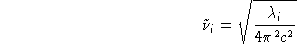
At this point, the eigenvalues need to be converted frequencies in units of reciprocal centimeters. First we change from frequencies ( ![]() ) to wavenumbers (
) to wavenumbers ( ![]() ), via the relationship
), via the relationship ![]() , where c is the speed of light. Solving
, where c is the speed of light. Solving ![]() for
for ![]() we get
we get
![]()
The rest is simply applying the appropriate conversion factors: from a single molecule to a mole, from hartrees to joules, and from atomic mass units to kilograms. For negative eigenvalues, we calculate ![]() using the absolute value of
using the absolute value of ![]() , then multiply by -1 to make the frequency negative (which flags it as imaginary). After this conversion, the frequencies are ready to be printed out.
, then multiply by -1 to make the frequency negative (which flags it as imaginary). After this conversion, the frequencies are ready to be printed out.
Calculate reduced mass, force constants and cartesian displacements
All the pieces are now in place to calculate the reduced mass, force constants and cartesian displacements. Combining Equation 6 and Equation 7, we arrive at
![]()
where ![]() is the matrix needed to diagonalize
is the matrix needed to diagonalize ![]() . Actually,
. Actually, ![]() is never calculated directly in Gaussian. Instead,
is never calculated directly in Gaussian. Instead, ![]() is calculated, where
is calculated, where ![]() is a diagonal matrix defined by:
is a diagonal matrix defined by:
![]()
and i runs over the x, y, and z coordinates for every atom. The individual elements of ![]() are given by:
are given by:
The column vectors of these elements, which are the normal modes in cartesian coordinates, are used in several ways. First of all, once normalized by the procedure described below, they are the displacements in cartesian coordinates. Secondly, they are useful for calculating a number of spectroscopic properties, including IR intensities, Raman activies, depolarizations and dipole and rotational strengths for VCD.
Normalization is a relatively straight forward process. Before it is printed out, each of the 3N elements of ![]() is scaled by normalization factor
is scaled by normalization factor ![]() , for that particular vibrational mode. The normalization is defined by:
, for that particular vibrational mode. The normalization is defined by:

The reduced mass ![]() for the vibrational mode is calculated in a similar fashion:
for the vibrational mode is calculated in a similar fashion:

Note that since ![]() is orthonormal, and we can (and do) choose
is orthonormal, and we can (and do) choose ![]() to be orthonormal, then
to be orthonormal, then ![]() is orthonormal as well. (Since
is orthonormal as well. (Since ![]() then
then ![]() ).
).
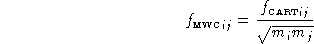
We now have enough information to explain the difference between the reduced mass Gaussian prints out, and the one calculated using the formula usually used for diatomics:
The difference is in the numerator of each term in the summation. Gaussian uses ![]() rather than 1. Using the elements of
rather than 1. Using the elements of ![]() yields the consistent results for polyatomic cases, and automatically takes symmetry into consideration. Simply extending the formula from Equation 14 to
yields the consistent results for polyatomic cases, and automatically takes symmetry into consideration. Simply extending the formula from Equation 14 to ![]() would (incorrectly) yield the same reduced mass for every mode of a polyatomic molecule.
would (incorrectly) yield the same reduced mass for every mode of a polyatomic molecule.
The effect of using the elements of ![]() in the numerator is to make the unit length of the coordinate system Gaussian uses be the normalized cartesian displacement. In other words, in the coordinate system that Gaussian uses, the sum of the squares of the cartesian displacements is 1. (You can check this in the output). In the more common coordinate system for diatomics, the unit length is a unit change in internuclear distance from the equilibrium value.
in the numerator is to make the unit length of the coordinate system Gaussian uses be the normalized cartesian displacement. In other words, in the coordinate system that Gaussian uses, the sum of the squares of the cartesian displacements is 1. (You can check this in the output). In the more common coordinate system for diatomics, the unit length is a unit change in internuclear distance from the equilibrium value.
One of the consequences of using this coordinate system is that force constants which you think should be equal are not. A simple example is H ![]() versus HD. Since the Hessian depends only on the electronic part of the Hamiltonian, you would expect the force constants to be the same for these to molecules. In fact, the force constant Gaussian prints out is different. The different masses of the atoms leads to a different set of Sayvetz conditions, which in turn, change the internal coordinate system the force constants are transformed to, and ultimately the resulting force constant.
versus HD. Since the Hessian depends only on the electronic part of the Hamiltonian, you would expect the force constants to be the same for these to molecules. In fact, the force constant Gaussian prints out is different. The different masses of the atoms leads to a different set of Sayvetz conditions, which in turn, change the internal coordinate system the force constants are transformed to, and ultimately the resulting force constant.
The coordinates used to calculate the force constants, the reduced mass and the cartesian displacements are all internally consistent. The force constants 


Summary
To summarize, the steps Gaussian uses to perform vibrational analysis are:
- Mass weight the Hessian
- Determine the principal axes of inertia

- Generate coordinates in the rotating and translating frame

- Transform the Hessian to internal coordinates and diagonalize


- Calculate the frequencies
- Calculate reduced mass, force constants and cartesian displacements
^{-1}")


A note about low frequencies
You’ll find that the frequencies for the translations are almost always extremely close to zero. The frequencies for rotations are quite a bit larger. So, how “close to zero” is close enough? For most methods (HF, MP2, etc.), you’d like the rotational frequencies to be around 10 wavenumbers or less. For methods which use numerical integration, like DFT, the frequencies should be less than a few tens of wavenumbers, say 50 or so.
If the frequencies for rotations are not close to zero, it may be a signal that you need to do a tighter optimization. There are a couple of ways to accomplish this. For most methods, you can use Opt=Tight or Opt=Verytight on the route card to specify that you’d like to use tighter convergence criteria. For DFT, you may also need to specify Int=Ultrafine, which uses a more accurate numerical integration grid.
As an example, I reran the water HF/3-21G* calculation above, with both Opt=Tight and Opt=VeryTight. You can see in Table 1 that the rotational frequencies are an order of magnitude better for Opt=Tight than they were for just Opt. Using Opt=Verytight makes them even better.
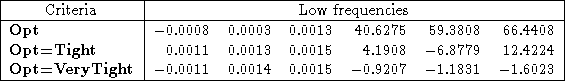
Table 1: The effect of optimization criteria on the low frequencies of water using HF/3-21G*. The frequencies are sorted by increasing absolute value, so that it’s easier to distinguish rotational modes from vibrational modes.
This raises the question of whether the you need to use tighter convergence. The answer is: it depends – different users will be interested in different results. There is a trade off between accuracy and speed. Using Opt=Tight or Int=Ultrafine makes the calulation take longer in addition to making the results more accurate. The default convergence criteria are set to give an accuracy good enough for most purposes without spending time to converge the results beyond this accuracy. You may find that you need to use the tighter criteria to compare to spectroscopic values, or to resolve a strucutre witha particularly flat potential energy surface.
In the water frequency calculation above, using tighter convergence criteria makes almost no difference in terms of energy or bond lengths, as Table 2 demonstrates. The energy is converged to less then 1 microHartree, and the OH bond length is converged to 0.0002 angstroms. Tightening up the convergence criteria is useful for getting a couple of extra digits of precision in the symmetric stretch frequency.
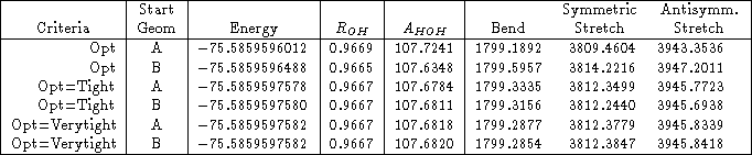
Table 2: The default optimization settings yield results accurate enough for most purposes. Tighter optimizations make almost no difference for this HF/3-21G* frequency calculation on water.
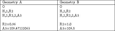
Table 3: Initial geometries for water optimization calculations. Geometry A was produced by Geom=ModelA. Geometry B is a slightly modified version of Geometry A.
You can also see that the final geometry parameters obtained with the default optimization criteria depend somewhat on the initial starting geometry. Using Opt=VeryTight all but eliminates these differences. I’ve included the starting geometries in Table 3, for those who wish to reproduce these results. (Using the default convergence criteria may give somewhat different results than those I’ve shown if you use a different machine, or even the same machine using different libraries or a different version of the compiler).
With DFT, Opt=VeryTight alone is not necessarily enough to converge the geometry to the point where the low frequencies are as close to zero as you would like. To demonstrate this, I have run B3LYP/3-21G* optimizations on water, starting with geometry B from Table 3, with Opt, Opt=Tight and Opt=VeryTight. The results are in Table 4. The low frequencies from these two jobs hardly change, and in fact get worse for the Tight and VeryTight optimizations.
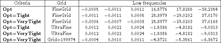
Table 4: The effect of grid size on the low frequencies from B3LYP/3-21G* on water with Opt, Opt=Tight and Opt=VeryTight. More accurate grids are necessary for a truly converged optimization. The frequencies are sorted by increasing absolute value, so that it’s easier to distinguish rotational modes from vibrational modes.
Given the straight forward convergence seen with Hartree-Fock theory, this might not seem to make sense. However, it does make sense if you recall that DFT is done using a numerical integration on a grid of points. The accuracy of the default grid is not high enough for computing low frequency modes very precisely. The solution is to use a more numerically accurate grid. The tighter the optimzation criteria, the more accurate the grid needs to be. As you can see in Table 4, increasinfg the convergence criteria from Tight to VeryTight without increasing the numerical accuracy of the grid yields no improvement in the low frequencies. For Opt=Tight, we recommend using the Ultrafine grid. This is a good combination to use for systems with hindered rotors, or if exact conformation is of concern. If still more accuaracy is necessary, then an unpruned 199974 grid can be used with Opt=VeryTight. Again, the higher accuracy comes at a higher cost in terms of CPU time. The VeryTight optimization with a 199974 grid is very expensive, even for medium sized molecules. The default grids are accurate enough for most purposes.
Acknowledgements
I’d like to thank John Montgomery for his constructive suggestions, Michael Frisch for clarifying several points, and H. Berny Schlegel for taking the time to discuss this material with me. Thanks also to Jim Cheeseman, for lending me his copy of Wilson, Decius and Cross.
Last updated on: 1 November 2021.