


This technical note discusses the procedure for transforming the UV/Visible numeric data computed by Gaussian into plots that are similar to what is observed experimentally. It is designed for people who want to understand how GaussView generates its UV/Visible plots and/or who want to generate their own spectra.
The output files from Gaussian excited states calculations report the excitation energies and oscillator strength for each excited state. For example, here is the output section for the first excited state from a TD-DFT calculation:
 Excited State   1:      Singlet-?Sym    5.4863 eV  284.45 nm  f=0.0002  <S**2>=0.000
      20 -> 22         0.49950
      21 -> 23         0.49950
 This state for optimization and/or second-order correction.
 Total Energy, E(TD-HF/TD-KS) =  -231.908393253
 Copying the excited state density for this state as the 1-particle RhoCI density.
Plots of the predicted UV/Visible spectrum for a molecule use this numeric data from each of the computed excited states.
Conventionally, UV-Visible spectra area plotted as ε vs. λ (excitation wavelength in nm), and the peaks assume a Gaussian band shape. The equation of a Gaussian band shape is:
[Equation 1]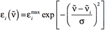
where the i subscript refers to the electronic excitation of interest. The other symbols have the following meanings:
- ṽi is the excitation energy (in wavenumbers) corresponding to the electronic excitation of interest.
- εimax is the value of εi at the maximum of the band: when the energy of the incident radiation ṽ is equal to ṽi.
- σ is the standard deviation in wavenumbers, which is related to the width of the simulated band. Specifically, it is the half-width of the Gaussian band at ε=εmax/e. Recall that wavenumbers are the reciprocal of wavelengths.
The relationship between εimax and the dipole strength (D) can be establish from the expression that relates D to ε and ṽ:
[Equation 2]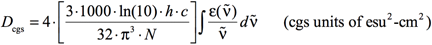
At the maximum of the band, this becomes:
[Equation 3]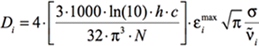
where again σ is the standard deviation (related to the width of the band). The other constants are well-known:
- Avogadro’s number: N = 6.02214199×10²³ mol-1
- The speed of light: c = 29979245800.0 cm·s-1
- Planck’s constant: h = 6.62606876×10⁻³⁴J sec = 6.62606876×10⁻³⁰ kg·cm2·sec-1
The factor of 1000 converts between cm3 and L.
The Gaussian output does not print the dipole strengths, Di, but instead reports the oscillator strengths,
fi, for each electronic transition. The relationship between these two quantities is given by the following equation:
[Equation 4]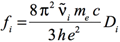
where fi is the (dimensionless) oscillator strength corresponding to the electronic excitation of interest, and Di
is the corresponding dipole strength in esu2 cm2. As before, ṽ is the corresponding excitation energy in wavenumbers. The remaining two constants are:
- The charge on the electron: e = 4.803204×10⁻¹⁰ esu
- The electron mass: me = 9.10938×10⁻³¹ kg
Using Equations 3 and 4, Equation 1 becomes:
[Equation 5]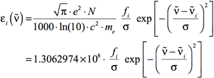
where εi is in units of L mol-1 cm-1, and σ is in cm-1. Note that the default in GaussView is σ = 0.4 eV.
As we saw earlier, the data for each predicted excited state appears in the Gaussian output file as follows:
Excited State 1: Singlet-?Sym 5.4863 eV 225.99 nm f=0.0002 <S**2>=0.000
The values from excited state 1 that are needed for generating the visualized spectrum are:
- The excitation energy in nm (red): λ1=225.99 nm
- The oscillator strength (blue): f1=0.0002
Using a value of 0.4 eV for the standard deviation—σ = 0.4 eV = 1/3099.6 nm-1 = 10-7/3099.6 cm-1—will result in the following equation:
[Equation 6]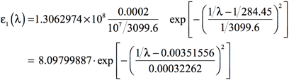
Plotting the results of Equation 6 for the range of frequencies of interest will yield the simulated spectrum. For example, if the region of the spectrum of interest is from 500 nm to 100 nm, one would use values of λ in this range.
In most cases, there will be more than one electronic excitation in the region of interest. In such cases, Equation 5 still provides the method for computing the shape of each individual band. The overall spectrum will come then from the sum of all the individual bands:
[Equation 7]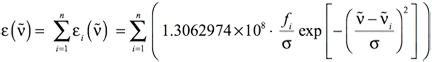
where i runs from the first to the nth electronic excitation, where n is the value set with the NStates=n option to the excited state method keyword (e.g., TD or EOM) in Gaussian.
Consider an example with three electronic excitations in the region of the spectrum of interest. The Gaussian output will provide values for each excited state. Here, we have extracted the first line of the output section for each excited state:
Excited State   1:      Singlet-A      4.3587 eV  284.45 nm  f=0.0002  <S**2>=0.000
Excited State   2:      Singlet-A      6.4307 eV  192.80 nm  f=0.5035  <S**2>=0.000
Excited State   3:      Singlet-A      8.0472 eV  154.07 nm  f=0.0061  <S**2>=0.000
This output yields the following values for use in simulating the spectrum:
- λ1=284.45, f1=0.0002
- λ2=192.80, f2=0.5035
- λ3=154.07, f3=0.0061
Using the same value for the standard deviation σ as previously—0.4 eV—will result in the following equation for the three bands:
[Equation 8]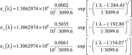
By adding the preceding three equations, we obtain the following expression for the simulated UV-Visible spectrum as the combination of the three bands computed by Gaussian:
[Equation 9]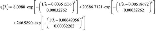
A spreadsheet program such as Excel or OpenOffice can be used to compute multiple values from the formulas above. For example, after computing the values ranging from 100 nm to 300 nm, at intervals of 10 nm, we obtain the following simulated UV-Visible spectrum:
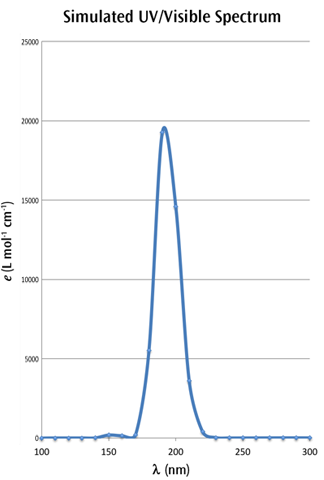
We have retained the markers for the individual points in the figure so that you can see how the curve was constructed.
Last updated on: 21 June 2017.