


One of the most important goals of a physical chemistry course is getting students to understand the relationship between a substances molecular structure and its physical properties. Laboratory experiments and exercises can serve an important role in conveying this concept by allowing students to explore these relationships for themselves and in detail.
In such investigations, electronic structure calculations can be used to introduce students to the importance of quantum mechanical effects. In this brief article, we discuss using the Gaussian program to study two geometric isomers of C10H8: naphthalene and azulene.
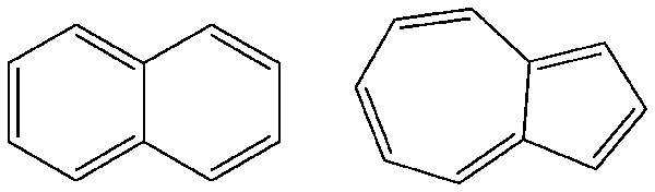
naphthalene azulene
Studying these Compounds in the Lab
Studying naphthalene and azulene is useful in that doing so allows students to compare the properties of two superficially similar molecules. A plausible first question to investigate is which isomer is more stable and why. This question can be approached experimentally by comparing the two heats of combustion, which can both be measured easily using a bomb calorimeter. A small-sized bomb makes this experiment practical even for a compound as expensive as azulene since a modest sample size (approximately 100 mg) can be used. (See the paper cited at the end of this article for details of the exact experimental procedures and several associated caveats.)
Figure 1. Sample Gaussian Input File
# RHF/6-31G(d) Opt Freq=ReadIso
Azulene
0 1
molecule specification
300 1.0 0.9135
isotopes in same order as molecule spec. (C=12,H=1)
Modeling Naphthalene and Azulene
These molecular systems also can be studied computationally using Gaussian, using either the PC running Windows or a UNIX workstation. In order to predict the relative stabilities of the two isomers, it is necessary to compute the absolute enthalpy for each molecule and then comparing these two values. This will involve performing a geometry optimization on each molecule to in order to determine the minimum energy structure, followed by a frequency calculation at the optimized geometry during which various thermochemical quantities are also computed.
This process is carried out using three different model chemistries: the AM1 semi-empirical model, the HF/6-31G(d) model (Hartree-Fock theory using a medium-sized basis set), and the B3LYP/6-31G(d) model (a hybrid density functional model again using a medium-sized basis set). The difference in absolute enthalpies is formally equivalent to the difference in heats of combustion since both compounds have the same empirical formula.
An abbreviated sample input file is given in Figure 1. In this file, we use the Opt Freq keyword combination to request a geometry optimization =immediately followed by a frequency calculation at the optimized geometry. The ReadIso option to the Freq keyword allows us to specify the temperature at which the frequencies should be predicted as well as some other parameters. The first line of the input section below the molecule specification contains the desired temperature (300 K), pressure (1 atmosphere) and scale factor (we use the standard value, which corrects for systemmatic error in frequency calculations), and subsequent lines give the desired isotope for each atom in the molecule (we select the standard isotope in all cases).
The output from this job is quite long, but the relevant results section is easy to find and is illustrated in Figure 2. The line labeled “Sum of electronic and thermal Energies” gives the predicted thermal-corrected energy for the molecule at the specified temperature (the value is printed in red). Below the list of energies is a breakdown of the thermal correction, divided into electronic, translational, rotational and vibrational components (highlighted in red in the sample output).
Figure 2. Sample Energy Results from the Calculation
Sum of electronic and zero-point Energies=        -385.757682
Sum of electronic and thermal Energies=           -385.750129
Sum of electronic and thermal Enthalpies=         -385.749179
Sum of electronic and thermal Free Energies=      -385.788191

            E (Thermal)            CV              S
             KCAL/MOL      CAL/MOL-KELVIN  CAL/MOL-KELVIN
TOTAL           89.483           32.274           81.601
ELECTRONIC        .000             .000             .000
TRANSLATIONAL     .894            2.981           40.486
ROTATIONAL        .894            2.981           26.207
VIBRATIONAL     87.695           26.312           14.908
Calculation Results
Table 1 presents the results of our calculations. In all cases, naphthalene is predicted to be the lower energy structure-and hence the more stablein agreement with experiment. Only the B3LYP/6-31G(d) model chemistry in is good quantitative agreement with the observed DH, differing from it by less than 2 kcal/mol (and within the experimental error bars). This indicates that the problem requires a model that includes the effects of electron correlation.
| Model | Energies | ||
|---|---|---|---|
| Napthalene (hartrees) |
Azulene (hartrees) |
DH(kcal/mol) | |
| AM1 | 0.21018 | 0.27764 | -42.33 |
| HF/6-31G(d) | -383.20359 | -383.13418 | -43.56 |
| B3LYP/6-31G(d) | -385.75013 | -385.69641 | -33.71 |
| Experimental | -35.3±2.2 | ||
Table 2 lists the CPU requirements for the various jobs in this study. As this data indicates, these jobs are all quite feasible on a UNIX workstation or a reasonably configured PC.
| CPU Time | (hrs:mins:secs) | |||
|---|---|---|---|---|
| Naphthalene | Azulene | |||
| Model | WSb | PCc | WSb | PCc |
| AM1 | 0:00:13 | 0:01:46 | 0:00:18 | 0:02:19d |
| HF | 0:56:14 | 1:59:04 | 1:37:26 | 3:00:25d |
| B3LYP | 1:03:46 | 2:20:02 | 2:11:28 | 4:30:00d |
a Default memory size used for all jobs
b IBM RS/6000 Power3 workstation with 1024 MB memory
c Pentium II processor (400MHz) with 256 MB memory
d Estimate based on the naphthalene ratio
Benefits to Students
In conjunction with their experimental measurements, this exercise will help students to learn that energy differences between isomers can be measured and calculated. It will also acquaint them with simple electronic structure calculations and help them relate their results to actual observable physical properties.
Find Out More
For more information, see the article “Naphthalene and Azulene I: Semimicro Bomb Calorimetry and Quantum Mechanical Calculations,” Carl Salter and James B. Foresman, J. Chem. Ed., 75, 1341 (1998)
Last updated on: 21 June 2017.