


Selecting the method and basis set to use for a computational study almost always involves finding an effective tradeoff between desired accuracy—as high as possible—and the (finite) available computing resources. Unfortunately, high accuracy model chemistries scale unfavorably with the size of the molecule, resulting in a practical limit on how large a system can be studied, placing many systems of chemical and/or biological interest out of reach of traditional approaches.
Gaussian’s ONIOM method provides a means for overcoming these limitations. Originally developed by Morokuma and coworkers [Dapprich99], ONIOM first appeared in Gaussian 98, and several significant innovations in Gaussian 03 [Vreven03] make it applicable to much larger molecules. In Gaussian 16, ONIOM may be used to compute energies, perform geometry optimizations, and predict vibrational frequencies and electric and magnetic properties. Be aware that ONIOM energies are designed to be used in a relative manner only: i.e., for comparing values for reactants and products, for similar species, and the like (as for electronic structure energy values in general). Geometry optimizations and property and spectra predictions proceed in the same way as calculations using traditional ab initio methods. ONIOM results are reported the normal way within Gaussian output.
ONIOM stands for Our own N-layered Integrated molecular Orbital and molecular Mechanics. This computational technique models large molecules by defining two or three layers within the structure that are treated at different levels of accuracy. Calibration studies [Dapprich99, Vreven06a] have demonstrated that the resulting predictions are essentially equivalent to those that would be produced by the high accuracy method alone on the entire molecule.
ONIOM calculations can use a Molecular Mechanics method for the system as a whole and an ab initio one for the site of interest; such calculations are referred to as MO:MM calculations (indicating a molecular orbital method is combined with Molecular Mechanics) or as QM:MM (quantum mechanics with MM). Alternatively, two ab initio methods can be combined; in this case, the calculation type is called MO:MO.
The ONIOM method is applicable to large molecules in many areas of research, including enzyme reactions, reaction mechanisms for organic systems, cluster models of surfaces and surface reactions, photochemical processes of organic species, substituent effects and reactivity of organic and organometallic compounds, and homogeneous catalysis.
ONIOM Layers
In an ONIOM calculation, the molecular system under investigation is defined as 2 or 3 region—typically referred to as “layers”—which are modeled using successively more accurate model chemistries:
- The High Layer is the smallest one, and it is treated with the most accurate method. Bond formation and breaking takes place in this region. This layer is also called the Small Model System (SM). In a 2-layer ONIOM calculation, it is often simply called the Model System.
- The Low Layer consists of the entire molecule in a 2-layer ONIOM model. The calculation on this region corresponds to the environmental effects of the molecular environment on the site of interest (i.e., the high layer). The low layer is typically treated with an inexpensive model chemistry: molecular mechanics, a semi-empirical method, or an inexpensive ab initio method such a Hartree-Fock with a modest basis set.
- In a 3-layer ONIOM model, a Middle Layer is defined, and it is treated with a method that is intermediate in accuracy between the high level method and the low level method. This layer consists of a larger subset of the entire molecule than the Higher layer. It models the electronic effects of the molecular environment on the high layer. The combination of this layer along with the Low layer is referred to as the Intermediate Model System (IM).
The entire molecule is referred to as the Real System.
A First example
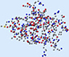
Figure 1 illustrates 2 (left) and 3-layer (right) ONIOM layer assignments in the resting state of oxidized ribonucleotide reductase (R2met; PDB file: 1XIK). The different visualization choices—wireframe, tube, and ball-and-stick—correspond to the low, medium and high layers (respectively).
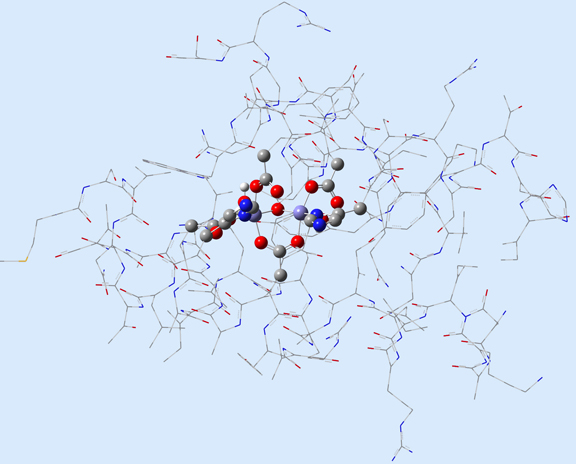
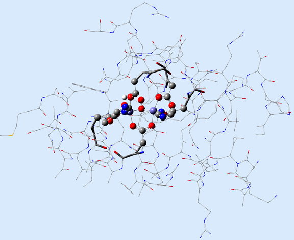
Figure 1. ONIOM Layer Definitions for Modeling Ribonucleotide Reductase [Torrent02]
Left: 2-layer ONIOM; Right: 3-layer ONIOM (H atoms not shown)
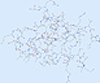
In this case, the researchers, Torrent, Morokuma and coworkers, defined the Real molecular system as 62 residues within the Fe-centered spheres of radii 18 Å (4 α-helical fragments). The active site becomes the high layer: specifically, the 2 Fe centers and the first shell ligands of 4 formates, 2 imidazoles and a few oxo, hydroxo and aquo groups. For the 3-layer ONIOM, the Intermediate Model is defined as the active site plus the side-chain and Cα atoms of the first coordinate shell. Figure 2 shows the three models as separate illustrations.
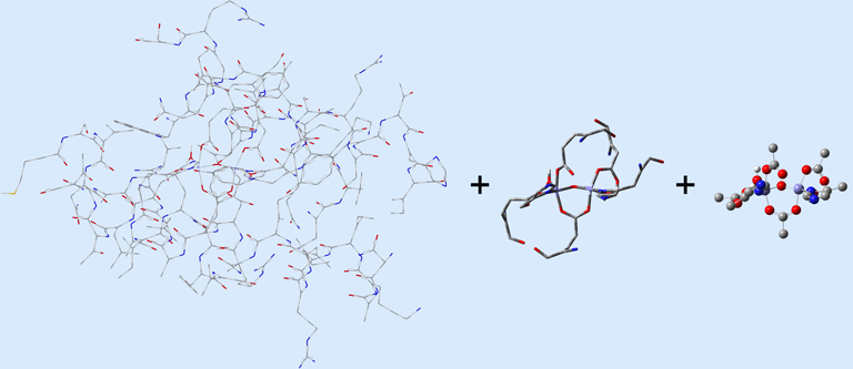
Figure 2. The Real, Intermediate Model and Small Model Systems
The results of conventional and ONIOM geometry optimizations on this system are presented in Table 1 (main chain atoms were fixed at their experimental positions for the ONIOM jobs) [Torrent02]. The final column in the table gives the RMS deviation for the structural parameters for the non-H atoms in the active site with respect to the experimental X-ray structure. As it indicates, the 2-layer ONIOM calculation cuts the error of the conventional calculation in half, illustrating the new insights made available by ONIOM. The 3-layer model results demonstrate that, for this case, considering the electronic effects of the protein residues improves the agreement with experiment.
| Optimization Job | Model Chemistry | #Atoms | RMS Dev. (Å) |
|---|---|---|---|
| DTF(active site only) | B3LYP/LANL2DZ | 43 | 0.62 |
| 2-layer ONIOM | B3LYP/LANL2DZ:Amber | 43:1034 | 0.34 |
| 3-layer ONIOM | B3LYP/LANL2DZ:HF/STO-3G:Amber | 43:88:1034 | 0.23 |
Figure 3 illustrates the improved agreement with experiment for the 2-layer ONIOM structure over the DFT geometry. In the illustration, the blue structure is the X-ray structure in both cases. The ONIOM geometry is drawn in green, and the B3LYP geometry is drawn in red. In the former, all of the active site atoms are in close proximity to their counterparts in the experimental structure, and the significant ring rotation with respect to the X-ray structure in the DFT results is eliminated.
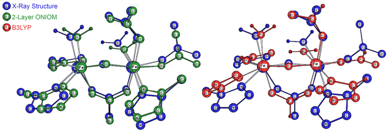
Figure 3. Comparison of the 2-Layer ONIOM (green, at left) and B3LYP
(red, on the right) Optimized Geometries with the Experimental X-Ray Structure (blue)
How ONIOM Works
The ONIOM method works by approximating the energy of the Real System as a combination of the energies computed by less computationally expensive means. Specifically, the energy is computed as the energy of the Small Model with corrections for the size difference between SM and R and for the method accuracy difference between the low level model chemistry and the high accuracy method used for SM (denoted low and high in the following equation):
Ehigh(R) ≈ Elow(SM) + {Elow(R) – Elow(SM)} + {Ehigh(SM) – Elow(SM)}
Size(SM → R) Level of Theory(low → high)
The preceding equation reduces to:
EONIOM = Elow(R) + Ehigh(SM) – Elow(SM)
Graphically, the computations for a 2-layer ONIOM calculation on the molecule mentioned previously proceed like this:
 |
≈ |  |
+ |  |
– | |
| DFT | Amber | DFT | Amber |
3-layer ONIOM calculations are performed in an analogous manner:
Ehigh(R) ≈ EONIOM = Elow(R) + Emedium(IM) + Ehigh(SM) – Elow(IM) – Emedium(SM)
|
≈ | |
+ |  |
+ | |
– | |
– | |
| DFT | Amber | HF | DFT | Amber | HF |
This scheme is a simplification of actual ONIOM procedures in Gaussian. In Gaussian 16, MO:MM ONIOM calculations can optionally take advantage of electronic embedding [Vreven06] within ONIOM calculations, which enables both the steric and electrostatic properties of the entire molecule to be taken into account when modeling processes in the high accuracy layer. This technique incorporates the partial charges of the MM region into the quantum mechanical Hamiltonian, thereby providing a better description of the electrostatic interaction between the QM and MM regions and allows the QM wave function to be polarized. ONIOM geometry optimizations can also optionally use a quadratic coupled (QC) algorithm which takes into account the coupling between atoms using internal coordinates (typically, those in the Small Model system) and those in Cartesian coordinates (typically, the atoms only in the MM layer) in order to produce more accurate steps. Note that optimizations using ONIOM proceed using the normal algorithms and procedures. ONIOM affects only the energy and gradient computations (ONIOM optimizations do not consist of independent, per-layer optimizations). The use of an integrated potential surface also enables vibrational analysis to be performed and related properties to be predicted.
Considerations for Defining Layers
The most important consideration when planning an ONIOM study is the selection of the various layers used in the calculation. The general principle to keep in mind is that the chemically active portion of the system should be included in the model system(s) and treated at the high level, while the remainder of the molecule can be treated at a low level in the Real system. Often, one knows by intuition what the most important part of the system is, and is thus able to define the ONIOM layers quite easily.
- Bond breaking or formation should not take place within the MM region.
- Atoms linked by double or triple bonds should be placed within the same ONIOM region. Similarly, region boundaries should not fall within aromatic rings. Figure 4 illustrates this principle with tyrosine, showing 2 possible appropriate Small Model systems as well as one inappropriate one.
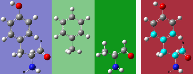
Figure 4.Tyrosine(left), two Possible Small Model Systems (green backgrounds), and an Incorrect Partitioning (far right). If any atom within the ring is chosen, then the entire ring must be part of the SM system. Similarly, if the carbon atom in the carbonyl is chosen, then the oxygen must be included as well. The highlighted atoms in the picture on the far right would not make an appropriate SM system as this partitioning violates both of the preceding constraints. Note that the two correct model systems have replaced C atoms in the Real system with H atoms. These are referred to as "link atoms," and they are discussed later in this article.
- In the case of a reaction, all Molecular Mechanics parameters must be the same within the Real and Model systems for both the reactants and the products. This ensures that the ONIOM results are independent of the definition of bonds and other coordinates within the reaction center. In general, to be completely safe, you must extend the SM system three bonds from any connectivity change. Sometime, however, this results in an SM system that is larger than is strictly necessary.
Figure 5 provides an example of the final principle. An SM which included only the Ni atom but not the P atom would result in different angular terms between the SM and Real systems (e.g., C-Ni-P vs.C-Ni-H). If you are not familiar enough with MM methodology to determine this by inspection, you can use the S-Value test to verify that your ONIOM partitioning avoids this pitfall (discussed in the next section). In this case, the test demonstrates that including additional atoms within the SM is not necessary.
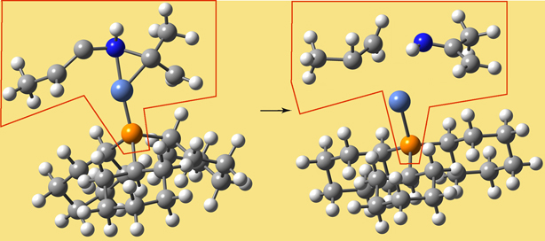
Figure 5. MM Partitioning Example. An appropriate Small Model for this reaction (indicated in red) must include both the Ni and P atoms. If the P atom is omitted, then several MM angular terms are defined differently within the reactant and the products (e.g., P-Ni-C vs. P-Ni-N).
References [Vreven06a, Morokuma01] discuss selecting the model system.
The S-Value Test
You can use the substituent value (S-Value) test [Vreven06a, Morokuma01, Vreven06] for two purposes:
- To verify the appropriateness of a potential ONIOM MO:MM partitioning scheme [Vreven06].
- To verify that the ONIOM approximation yields sufficient accuracy for a series of compounds to be studied [Morokuma01].
The S-Value is defined as the difference in E between the Model and Real systems at a certain level of theory. When used for the first purpose, the S-Value test involves MM computations which compare the energy differences between the Real and Model systems of the reactants’ bonding scheme to that of the products. For example, for the reaction in Figure 5, we would compute the MM energy for the Model and for the Real system using the bonding scheme of the reactants and that of the product, performing in this case 4 UFF calculations: the Real system for the reactants’ bonding scheme and product bonding scheme, and the Model system for the same two systems:
ΔS-ValueMM partitioning = {EUFF(react.-bonds,R) – EUFF(react.-bonds,SM)} – {EUFF(prod.-bonds,R) – EUFF(prod.-bonds,SM)}
You can accomplish this using 2 ONIOM(UFF:UFF) calculations (discussed under "Sample Output" below). Once the jobs are complete, the energy difference between the Model and Real system is computed for both bonding schemes.
Table 2 summarizes the results of the S-Value test for the appropriate SM shown in Figure 5 and for an alternative SM which omits the P atoms. Note that the energy difference is the same for the two molecular systems when the P atom is included in the SM and very different when it is not, indicating that the correct SM is the one in Figure 5.
| Bonds as in the… | SM | Real | S-Value |
|---|---|---|---|
| Reactants: P in MM only | 0.48849 | 0.71378 | 0.22529 |
| Product: P in MM only | 0.11158 | 0.19048 | 0.07891 |
| Reactants: P in SM | 0.65572 | 0.71278 | 0.05806 |
| Product: P in SM | 0.13242 | 0.19048 | 0.05806 |
See reference [Vreven06] for a detailed example of performing an S-Value test like this one.
Be aware that an S-Value test such as this one confirms only that the proper SM has been chosen. It is still an open question whether ONIOM is an appropriate method for studying the system. This question is addressed by a different sort of S-Value test.
The second use of the S-Value test is to determine whether the ONIOM procedure is a valid approximation for the desired high accuracy model chemistry. Doing so involves comparing the high accuracy and low accuracy methods’ energy difference between the Real system and the Model system:
ΔS-ValueONIOM approx. = {Ehigh(R)–Ehigh(SM)} – {Elow(R)–Elow(SM)}
Determining the S-Value will thus require 4 calculations: 2 on the Real system and 2 on the Small Model system, using the target accuracy method and the low level method in each case. This can be accomplished in 2 Gaussian jobs, however, as the program includes a facility to compute the S-Value (discussed below).
Although the S-Value test is computationally expensive—since it involves running the high accuracy calculation that you were trying to avoid by using ONIOM in the first place—it is nevertheless useful for verifying ONIOM’s appropriateness when you want to apply the method to a series of compounds. The S-Value test can be performed on 2 small, representative systems. Comparing the S-Values for the two systems will allow you to determine whether the ONIOM approach is viable for that series of compounds; if they differ significantly, then using ONIOM is not advisable.
Link Atoms
In the course of an ONIOM calculation, atoms at the Model/Real system boundary—specifically, heavy atoms in the Real system which are bonded to atoms in the SM system—are modeled using link atoms when computations are performed on the SM system. For example, a carbon atom which is bonded to another carbon within the SM system is typically replaced by a hydrogen in the computations. The following diagram illustrates link atoms, using ethane as an example:
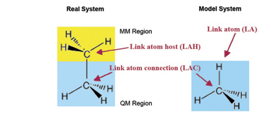
Link atoms must be included within the molecule specification for a Gaussian job (discussed later).
Setting up ONIOM Calculations in Gaussian
There are several unique aspects to setting up an input file for a Gaussian ONIOM calculation: specifying the route, including layer assignments and other information with the molecule, and optionally specifying per-layer charges and spin multiplicities. However, other than these items, ONIOM input is no different from that for regular calculations of the same type.
The ONIOM Keyword
ONIOM calculations are requested with the ONIOM keyword. The two or three desired model chemistries are specified as the options to the ONIOM keyword, in the order High, Medium, Low for a 3-layer ONIOM or High, Low for a 2-layer ONIOM. The distinct models are separated by colons. For example, this route section specifies a three-layer ONIOM calculation, using UFF for the Low layer, AM1 for the Medium layer, and HF for the High layer:
# ONIOM(HF/6-31G(d):AM1:UFF)
To perform a calculation to be included in an S-Value test, include the SValue option in the route section using the following syntax:
# ONIOM(B3LYP/6-31G(d):Amber)=SValue
Note that the SValue option is limited to single point energy calculations.
ONIOM Layers within the Molecule Specification
Atom layer assignment is done as part of the molecule specification, via additional parameters on each line according to the following syntax:
atom coordinates layer [link-atom [bonded-to [scale-fac1 [scale-fac2 [scale-fac3]]]]]
where atom and coordinates represent the normal molecule specification input for the atom (coordinates can be either Cartesian or internal coordinates). Note that when a Molecular Mechanics method is in use, then any required parameters (e.g., atom types and partial charges) must also be included in the atom specification.
Layer is a keyword indicating the layer assignment for the atom, one of High, Medium and Low; these may be abbreviated to their initial letter.
The other optional parameters specify how the atoms located at a layer boundary are to be treated. You use link-atom to specify the atom with which to replace the current atom (it can include atom type and partial charge and other parameters). Link atoms are necessary when covalent bonding exists between atoms in different layers in order to saturate the (otherwise) dangling bonds.
The bonded-to parameter specifies which atom the current atom is to be bonded to during the higher-level calculation portion. If it is omitted, Gaussian will attempt to identify it automatically. The three additional optional parameters are scale factors which affect the specifics of the calculation. See the ONIOM keyword discussion in the Gaussian 16 User’s Reference for details on their meanings and use.
Here are some example lines from molecule specifications for which we’ve labeled the various components:
Atom         Cartesian coordinates                  Layer
 C            0  -3.326965 0.607871 -0.778723      H
Atom-Type-Charge                Cartesian coordinates                       Layer            Link atom        LA Bonded to
C-CA--0.25        0  -4.748381  0.578498 -0.778569 H
C-CA--0.25        0  -5.419886 -0.619477 -0.778859 L          H-HC-0.1    5
The second section shows lines that could be used for an ONIOM calculation using Amber as the MM method; note how the atom specifications—for both the atom itself and the link atom—include the Amber atom type and partial charge. The final item in last line specifies which atom the LA is bonded to, indicated by a number indicating its position within the molecule specification (i.e., the fifth atom).
Per-Layer Charges and Spin Multiplicities
Multiple charge and spin multiplicity pairs may also be specified for ONIOM calculations. For two-layer ONIOM jobs, the format for this input line is:
chargelow(R) spinlow(R) chargehigh(SM) spinhigh(SM) chargelow(SM) spinlow(SM) [ chargehigh(R) spinhigh(R) ]
where the superscript indicates the model chemistry and the parameter the layer for which the value will be used. The fourth pair applies only to ONIOM=SValue calculations. When only a single value pair is specified, all levels will use those values. If two pairs of values are included, then the third pair defaults to the same values as in the second pair. If the final pair is omitted for an S-Value job, it defaults to the values for the real system at the low level.
Values and defaults for three-layer ONIOM calculations follow an analogous pattern. See the ONIOM keyword in the Gaussian 16 User’s Reference for full details.
Input Examples
Here is a simple ONIOM input file:
# ONIOM(B3LYP/6-31G(d,p):AM1:UFF) Opt Test

ONIOM optimization

0 1
C  0   -0.6623  0.0002 -0.2895 L
H  0   -0.0522 -0.9047 -0.0512 L
H  0   -0.0520  0.9051 -0.0513 L
C  0   -1.6365  0.0005  0.9031 L H
C  0   -0.5617  0.0004  1.9498 H
H  0   -2.2867 -0.9043  0.8225 L
H  0   -2.2865  0.9054  0.8224 L
H  0   -1.0072  0.0006  2.9742 H
H  0    0.0856 -0.9046  1.8511 H
H  0    0.0859  0.9052  1.8509 H
H  0   -1.0698  0.0002 -1.7334 L
Here is an input file created with GaussView that includes the additional input required for the Amber MM method. It also illustrates the use of per-layer charges and spin multiplicities:
# ONIOM(B3LYP/6-31G(d):Amber) Geom=Connectivity

2 layer ONIOM job

0 1 0 1 0 1
C-CA--0.25  0   -4.703834    -1.841116    -0.779093 L
C-CA--0.25  0   -3.331033    -1.841116    -0.779093 L H-HA-0.1  3
C-CA--0.25  0   -2.609095    -0.615995    -0.779093 H
C-CA--0.25  0   -3.326965     0.607871    -0.778723 H
C-CA--0.25  0   -4.748381     0.578498    -0.778569 H
C-CA--0.25  0   -5.419886    -0.619477    -0.778859 L H-HC-0.1  5
H-HA-0.1    0   -0.640022    -1.540960    -0.779336 L
H-HA-0.1    0   -5.264565    -2.787462    -0.779173 L
H-HA-0.1    0   -2.766244    -2.785438    -0.779321 L
C-CA--0.25  0   -1.187368    -0.586452    -0.779356 L H-HA-0.1  3
C-CA--0.25  0   -2.604215     1.832597    -0.778608 H
H-HA-0.1    0   -5.295622     1.532954    -0.778487 H
H-HA-0.1    0   -6.519523    -0.645844    -0.778757 L
C-CA--0.25  0   -1.231354     1.832665    -0.778881 L H-HC-0.1  11
C-CA--0.25  0   -0.515342     0.610773    -0.779340 L
H-HA-0.1    0   -3.168671     2.777138    -0.778348 H
H-HA-0.1    0   -0.670662     2.778996    -0.779059 L
H-HA-0.1    0    0.584286     0.637238    -0.779522 L

1 2 1.5 6 1.5 8 1.0
2 3 1.5 9 1.0
3 4 1.5 10 1.5
...
17
18
Using Gaussian to define ONIOM Layers
Choosing the Edit=>Select Layer menu item or clicking on the Select Layer button opens the Layer Selection Tool. This window is used to assign atoms to ONIOM layers graphically. It is illustrated in Figure 6.
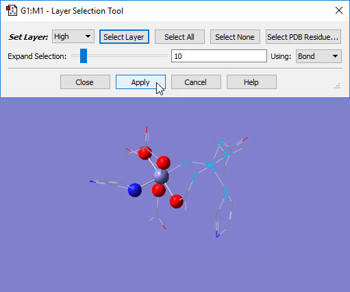
Figure 6. Assigning Atoms to ONIOM Layers in GaussView.
The selected atoms are about to be placed into the High layer (i.e., the SM system).
This dialog allows you to assign atoms to layers for ONIOM calculations. Different layers are indicated by the different display formats. Here, several atoms are selected for layer assignment.
There are several methods for selecting atoms for layer assignment:
- You can use one of the buttons at the top of the dialog. The All button selects all atoms in the molecule, and the None button deselects all atoms. The Layer button selects all atoms currently assigned to the specified layer. The Select PDB Group opens another selection dialog, shown in Figure 7, which allows you to select atoms by residue if this information was present in the PDB file corresponding to the current model. This dialog allows you to specify the desired residue by residue name (type), residue number and/or chain (A or B). Omitted items act as wildcards. For example, if you enter only residue number 5, then residue 5 in both chains will be selected. Similarly, entering only a residue name will cause all residues of that type within the molecule to be selected.
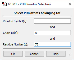
Figure 7. Selecting Atoms for Layer Assignment by PDB Residue
- Use the left mouse button to select or deselect atoms manually, continuing until all the atoms that you want have been selected. Hold down the Shift key to add to the current selection.
- Proximity-based selection: Select an atom, and then use the Expand Selection slider and proceed until you have selected all the atoms you need. Moving it to the right increases the distance used when selecting atoms.
For distance based atom selection, the distance between atoms to be selected depends on the following criteria, selected in the Using popup menu:
- Bond, which selects only atoms that are bonded.
- Distance, which selects an atom based solely on proximity to a current selection, regardless of whether or not it is bonded.
Once atoms are selected, you must click on the Apply button to assign them to that layer. Clicking on Apply turns off the selection.
By default, atoms in different layers are displayed in different formats in the view window. Using the standard settings, atoms in the High layer appear in ball-and-stick format, atoms in the Medium layer are displayed as tubes, and atoms in the Low layer are in wireframe format. These can be customized via the corresponding fields in the Molecule panel of the Display Format preferences.
Sample ONIOM Output
Energies and other properties computed with ONIOM appear in the normal way within Gaussian output. In addition, the energies for the component calculations are also reported, as in this example:
ONIOM: gridpoint  1 method:  low   system:  model energy:     0.002472457878
ONIOM: gridpoint  2 method:  high  system:  model energy:   -39.975899382065
ONIOM: gridpoint  3 method:  low   system:  real  energy:     0.005685659971
ONIOM: extrapolated energy = -39.972686179972
The first three lines give the energies for R at the low accuracy method, R at the high accuracy method and SM at the low accuracy method. The final line gives the ONIOM total energy.
If you are running an ONIOM calculation with a MM method specified for both layers, then these output lines will provide the energy values that you need to compute the S-Value (note that you don’t need to use the SValue option when verifying the layer partitioning for an MO:MM calculation). The first two lines (i.e., those labeled gridpoint 1 and 2) represent the same calculation and hence report the same energy, MM on the SM system, while the third line gives the energy for the Real system. Their difference can be computed and compared to the value for the other reaction component, which will indicate whether the MM region is properly defined.
For ONIOM=SValue calculations, some additional output is present:
S-Values (between gridpoints) and energies:

    high     2      -38.816693     4
         -39.975899            -78.792592
     low     1        0.003213     3
           0.002472              0.005686
                 model                  real
  ONIOM: gridpoint  1 method:  low   system:  model energy:     0.002472457878
  ONIOM: gridpoint  2 method:  high  system:  model energy:   -39.975899382065
  ONIOM: gridpoint  3 method:  low   system:  real  energy:     0.005685659971
  ONIOM: extrapolated energy =  -39.972686179972  diff=  -38.819905899363
The computed S-Value is highlighted in green in the output. This value can be compared to the one for a comparable system in order to verify that ONIOM models such systems in a consistent manner.
Two Example ONIOM Studies
In this final section, we will look at some research incorporating ONIOM studies by Bernd Goldfuss, Frank Rominger and Thomas Löschmann at the Organic Chemistry Institute of the University of Heidelberg [Goldfuss00, Goldfuss01] (Prof. Goldfuss is now at the University of Köln). These studies were investigating components related to synthesizing pharmaceutical products and chiral ligands in asymmetric catalysis. Their work combines synthesis and computational studies.
Axially chiral biaryls are important to pharmacological natural products and as chiral ligands in asymmetric catalysis. Successful enantioselective syntheses require the control of the biaryl axis in these compounds, which is a challenging problem. Fenchyl alcohols have been successfully used as precatalysts in enantioselective diethylzinc additions to benzaldehyde. These researchers consider the question of whether the fenchyl alcohol moiety can serve the same purpose in biphenyl derivatives (by inducing/stabilizing asymmetry at the biaryl axis).
Goldfuss and Rominger synthesized 2,2′-bis-((1R,2R,4S)-2-hydroxy-1,3,3-trimethylbicyclo[2.2.1]hept-2-yl)-1,1′-biphenyl (designated molecule 3 in [Goldfuss00]) by addition of 2,2’-dilithiobiphenyl to ()-fenchone. They found that its X-ray structure revealed an R-sense of asymmetry at the biphenyl axis (see Figure 8). It also indicated intramolecular hydrogen bonds between the hydroxy groups: O-H-OH at 2.2 Å and O-O at 3.0 Å.
Figure 8. Molecule 3-R from Reference [Goldfuss00]
They performed ONIOM calculations on the R and S forms of this compound in order to explore the origin of atropisomerism in S, optimized gas phase structures of R and S enantiomers. Their specific method was ONIOM(B3LYP/6-311++G(d,p):AM1). The SM consisted of the hydroxy groups. Their calculations indicated that the 3-R form was more stable than the 3-S form by a little over 6 kcal/mol.
The researchers state that the destabilization of 3-S with respect to 3-R is due to repulsion between methyl substituents of the bicyclohexane moities. 3-R is stabilized by favorable alignment of the bicycloheptane moities which support hydrogen bonding between the 2,2′-fenchyl alcohol units. Thus, the compound may be useful as a chiral ligand and host to form clathrates with organic guest molecules.
A second study by all three researchers focused an important class of reactions in this same area involving enantiopure organophosphorus compounds [Goldfuss01]. They attempted to synthesize the chiral, cleating phosphinofenchol 1 by adding 2-litho (diphenylphosphino)benzene to (-)-fenchone (Y=PPh2, X=H). However, the result was compound 2 rather than compound 1.
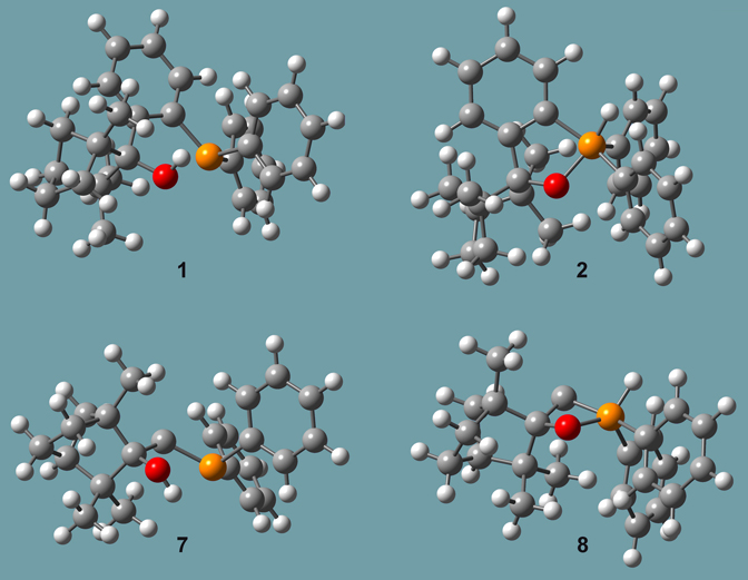
Figure 9. Molecules from Reference [Goldfuss01]
Other, similar pairs of species were also studied, including compounds 7 and 8 in Figure 9, as well as two more compounds where the hydrogen in the hydroxyl group/phosphorus atom is replaced by a methyl group (designed 9 and 10 in the paper). The reaction of lithiomethyl (diphenyl) phosphine with (-)-fenchone yielded compound 7 (and not 8, the structural analogue to 2). In contrast, the lithiation of the P-H group in 2 with nBuLi and subsequent reaction with methyliodide yields 10.
They performed ONIOM studies of these compounds, as well as the related systems 7 and 8 (also included in Figure 9), in which the phenyl bonded phosphorus atom is not present. Figure 10 illustrates the SM selection scheme for all of these calculations (using compound 7 as an example). The results of their synthetic and computational studies are summarized in Table 3.
Table 3. Synthesis and Relative Energy Results
| Coumpounds | Synthesis Yields | ΔEZPE-corrected | 1 vs.2 | 2 | -19.3 Kcal/mol |
|---|---|---|
| 7 vs.8 | 7 | +40.9 Kcal/mol |
| 9 vs.10 | 10 | -17.1 Kcal/mol |
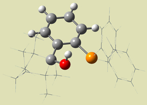
Figure 10. ONIOM Layer Scheme [Goldfuss01]
Given the energetics, the first and third results are surprising. The computational results suggest higher thermodynamic stabilities of open phosphines relative to cyclic phosphoranes. The formation of the metastable phosphoranes can be rationalized by considering these reactions focusing on the chemistry of the active site:
H3COH + H3CPH2↔ H3COPH3CH3 +19.4 kcal/mol
H3CO(–) + H3CPH2↔ H3COPH2(–)CH3 -9.9 kcal/mol
B3LYP/6-31+G(d) calculations for these reactions result in the indicated reaction energies. The formation of phosphorane from methanol and methylphosphine is disfavored by almost 20 kcal/mol, while the formation of phosphoranide from the addition of methanolate to methylphosphine is stable, with a ΔE of almost 10 kcal/mol with respect to the reactants. This difference can be rationalized by the better accommodation of negative charge in the latter case due to polarization, illustrated by the plot of the HOMO phosphoranide in Figure 11.
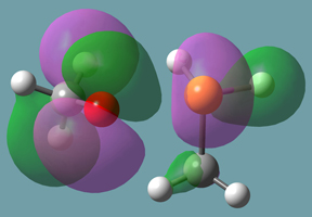
Figure 11. HOMO of Phosphoranide
Further Reading About ONIOM
We recommend starting with reference [Vreven06] below in order to take the next step in learning about ONIOM. It contains detailed information about performing MO:MM calculations. References [Dapprich99, Vreven03] provide information about the theory underlying ONIOM and its implementation in Gaussian 16. [Vreven06a, Morokuma01, Torrent02] provide further example applications, while [Morokuma01] also contains a detailed discussion of ONIOM in the context of traditional model chemistries, including calibration data. References [Goldfuss00, Goldfuss01] are the original studies by Goldfuss, Rominger and coworkers; they contain additional work, including many details of syntheses, which are not discussed here.
Last updated on: 21 June 2017.