


This note lists the new features in GaussView version 6.1.1, discussing changes with respect to version 6.0. Version 6.1.1 also includes many bug fixes and documentation clarifications.
Topics:
- Enhanced Spectra Mixture Editor
- Enhanced GMMX Conformational Searching
- New Preference for Mouse Hover Behavior
- Changes for G16 Features: Gaussian Calculation Setup and Others
- Additional Information in the Calculation Summary
- Enhancements to Spectra Facility
- Citation
- Displaying NMR Chemical Shifts
- Preferences for the Dipole Moment Vector Display
- Job Requirements for Displaying the Solvation Cavity
Enhanced Spectra Mixture Editor
This version of GaussView includes an greatly enhanced facility for displaying multiple spectra on a single plot. This feature is controlled via the Mixture Editor.
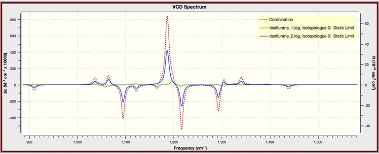
Example Spectra Plot for Multiple Data Sets
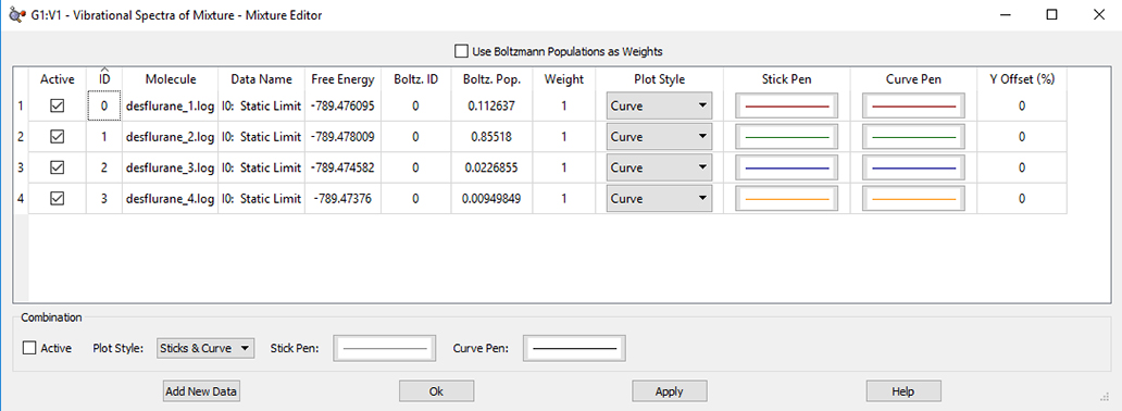
The Mixture Editor
The Mixture Editor dialog is used to modify plots when more than one data set is plotted. The dialog contains two sections:
- The spreadsheet-like list contains controls for each available data set. The list may be sorted by clicking on any column header. You can select multiple data sets using the control command and shift keys. Any changes made will apply to all selected items.
- The Combination region below the list contains the options for modifying the plot line corresponding to the combined and (possibly) weighted data.
The leftmost columns in the file list are as follows:
- : Whether the data set is included in the plot. Inactive data does not contribute Boltzmann Populations calculations. For the combination plot, the Active box controls whether this data is considered when GaussView determines plot scaling. The presence of the Combination data is controlled by its Plot Style (None hides it).
- : This displays the identification number given to the file. Numbering starts at 0. This column may be used to restore the original ordering.
- : This displays the name of the output file.
- : Contains a string describing the data set (used for plot legends). This may be edited.
- : This displays the free energy of the molecule. The units for this field are hartrees. When free energies are not available, the label changes to Energy and the field displays the total energy.
- : Identification number for the set’s Boltzmann group (see below). IDs start at 0.
- : This displays the conformer’s contribution to the Boltzmann population.
- : This displays the weight given to each molecule’s data in the plot. By default, GaussView will weight all data sets at 1. These values can be edited.
- : See below.
- : This option allows you to shift the Y-axis for the data by the amount you specify, expressed as a percentage.
Checking the box will set Boltzmann weighting for all items and remove column from table. Right-clicking within the file list brings up a menu with the following options which also modify the values in the Weight column:
- : Copy the Boltzmann populations into the column (where they may be edited).
- : Assigns each data set a weight of 1.0 (restoring it to the GaussView default).
- : Assigns each data set an equal weight that is normalized over all data sets.
Boltzmann Populations are computed from all data sets having the Boltzmann ID, including ones with set to . Vibration data of isomers (including nuclear mass) that match the same incident frequency from a Boltzmann group. Harmonic and anharmonic data are in different groups. This field is editable to allow you to redefine Boltzmann groups.
The data list below shows 2 Boltzmann groups:
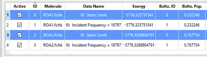 Boltzmann Groups: Static Limit (0) and 18797nm(1)
The following controls are located in both the Combination area and in each data set row:
- The Plot Style menu determines how the corresponding line is displayed. For the combination plot, the default style is (it is not visible); the default for the individual data sets is which displays as both Stick (plotted as pillars) and Curve (a sloped line connecting each of the plot points).
- The Stick Pen option allows you to customize the display when the Stick or Sticks and Curve options are selected. It has options to change the color, width, and line style (see below).
- The Curve Pen option allows you to customize the line displayed when the Curve or Sticks and Curve option are selected. It has options to change the color, width, and line style (see below).
On the bottom of this dialog, the Add New Data button allows you to add more data to the current plot, and it opens the OS default file opening system. The OK button will close the Mixture Editor dialog, and the Apply button will apply all changes you have made to the plot without closing the dialog.
Additional information about customizing multi-spectra plots can be found in the GaussView help.
Enhanced GMMX Conformational Searching
Many enhancements have been made to the internal algorithms of the add-on GMMX Conformational Search facilty. As a results, some of the controls in the corresponding dialog now operate differently:
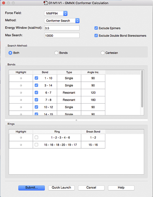
Setting up a GMMX Calculation
The Force Field dropdown menu allows you to choose what type of force field to use for the Conformer Calculation. The default force field is MMFF94, a general purpose organic force field designed primarily for
small, drug like organic molecules. The other two force fields, MMX and MM3, come from the Allinger group and differ from MMFF94 in the treatment of extended conjugation.
The Method dropdown menu specifies what kind of calculation to run:
- : Perform a conformational search based on the parameters specified in the dialog.
- : Optimize the current structure with molecular mechanics.
- : Perform a systematic conformational search in torsion space. The selected rotatable bonds are all set to an initial configuration and then stepped by the specified bond angle through 360 degrees. At each step, the current structure is minimized.
The Energy Window field specifies the tolerance level of the energy difference between the
results and the lowest energy conformer (in kcal/mol). When the calculation is run, conformers that fall outside of this range will be discarded.
The Max Search field specifies the maximum number of structures that will be minimized.
When checked, the Exclude Epimers checkbox says to remove all epimers of the current structutre from the results set. Epimers are stereoisomers whose configurations differ only at a single stereo center.
When checked, the Exclude Double Bond Stereoisomers checkbox will remove stereoisomers resulting from rotations around a double bond from the results set, with the exception of double bonds selected in the list. Rotations about the latter are always considered regardless of this setting.
For more information about GMMX and its procedures, see the GaussView help.
New Preference for Mouse Hover Behavior
In previous versions of GaussView, hovering the mouse over an atom would display its atom number and element type in the lower left corner of the View window (after a brief delay):
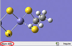
Mouse Cursor Tracking (Hovering)
This feature is known as mouse cursor tracking. It is now configurable using the Windows Behavior Preference panel:

The Windows Behavior Preference
The default behavior in GV 6.1.1 is to display this information only when the F5 key is held down. You can have it occur always or never with the other menu options.
Changes for G16 Features: Gaussian Calculation Setup and Others
There have been some additions to the Gaussian Calculation Setup dialog to support new Gaussian 16 features.
The Method panel has an popup which allows you to specify an empirical dispersion scheme for DFT calculations.
The %KJob Link 0 command can now be specified on the Link 0 panel.
In the Pop. panel, options for Merz-Kollman electrostatic potential-derived charges and minimum basis set set Mulliken charges have been added. Options for NBO7 have been added to the Perform NBO calc popup.
The Preview panel’s appearance can now be customized via items on its context (right click) menu:
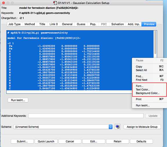
Customizing the Preview Panel
The Gaussian testrt utility, which checks the validity of the input file route section, can be run from the Preview panel using the corresponding button (below the input file display on the left). Doing so will produce testrt output in a separate window:
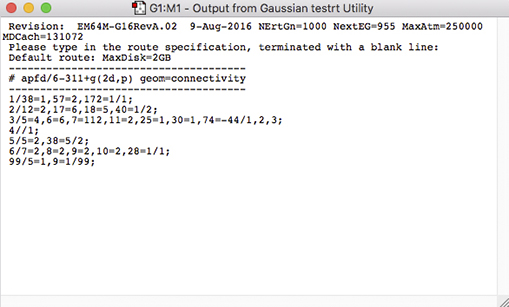
Output from testst
Several minor changes were also made to this dialog (see “GCS Item-G16 Keyword Equivalences” in the GaussView help):
- For the and job types, the Save Normal Modes checkbox has been converted to the pop-up menu.
- For the job type, the spin-spin coupling options have been collected into the popup menu.
- In the Pop. panel, the Save charges for later MM popup item has been renamed to .
In addition, the Redundant Coordinate Editor has been enhanced to match supported features in G16.
Additional Information in the Calculation Summary
The Gaussian Calculation Summary dialog’s Overview panel has some additional fields, as indicated by red stars in the following illustration:
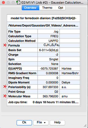
Overview Results from a Gaussian Calculation
Enhancements to Spectra Facility
For harmonic and anharmonic vibrational analysis results, the item on the
There is full support for Raman and ROA spectra: static and frequency-dependent, harmonic and anharmonic, and retrieved from log files or checkpoint files.
There is new labeling of Y axes for plots including intensity and scattering activities so that harmonic and anharmonic spectra can be compared directly.
Citation
You can cite GaussView version 6.1.1 as follows:
GaussView, Version 6.1.1, Roy Dennington, Todd Keith, and John Millam, Semichem Inc., Shawnee Mission, KS, 2019.
Displaying NMR Chemical Shifts
In the NMR Results dialog, the Shielding field displays the shielding value for the selected atom and set of reference values, which is used to compute the chemical shifts.
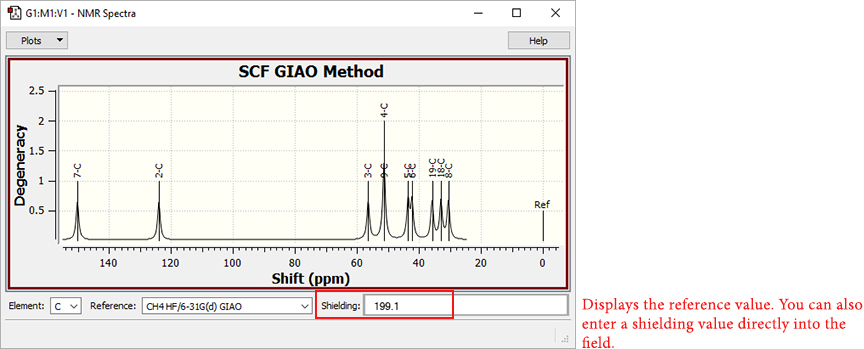
Visualizing Chemical Shifts
You can also type a value directly into the field. Although GaussView has had this capability for some time, it was not previously documented. Input values do not modify values in the reference set, and they cannot be saved.
Preferences for the Dipole Moment Vector Display
The Change Distribution Preferences panel now allows you to specify defaults for the color and thickness (radius) of the dipole moment vector display requested in the Display Charge Distribution dialog ():
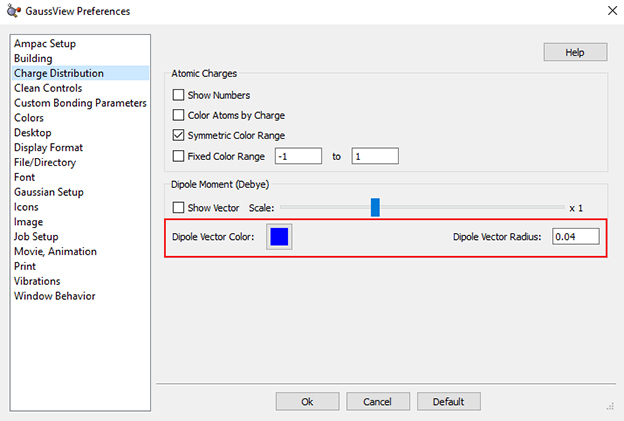
Dipole Moment Vector Display Preferences
Job Requirements for Displaying the Solvation Cavity
GaussView’s solvation cavity display feature requires that the Gaussian job be run with the SCRF=Read Gaussian route section option and that the input file include the PrintSpheres within the SCRF additional input section. Previous documentation referred to the PDens SCRF input item.
Last updated: 10 February 2020